ERA- Irrigation in East Africa

Author

Namita Joshi,, Todd Rosenstock & Peter Steward (Alliance of Bioversity International & CIAT)

Published

June 11, 2025

1 What is ERA?

1.1 Introduction

The Evidence for Resilient Agriculture (ERA) initiative was launched in 2012 to address the need for a robust evidence base on how agricultural practices perform under different conditions. Originally developed to evaluate the outcomes of Climate-Smart Agriculture (CSA), ERA has since evolved to include a wide range of technologies and practices relevant to agroecology, regenerative agriculture, ecosystem-based adaptation, and nature-based solutions.

ERA provides a large, structured meta-dataset of agricultural experiments, harmonized using a common data model and controlled vocabulary. The current version of the dataset (version = r era_version) includes r ERA_Compiled[,.N] observations from r ERA_Compiled[,length(unique(Code))] peer-reviewed agricultural studies conducted in Africa between r ERA_Compiled[,min(M.Year.Start,na.rm=T)] and r ERA_Compiled[!M.Year.End>2050,max(M.Year.End,na.rm=T)]. These observations cover more than r ERA_Compiled[,length(unique(PrName))] unique combinations of practices, and assess their effects on over r ERA_Compiled[,length(unique(Out.SubInd))] outcome indicators, including yield, soil health, and emissions.

Experiments were identified through systematic searches in Web of Science and Scopus and were screened against predefined criteria: geographic location, technology and outcome relevance, inclusion of both conventional and alternative treatments, and availability of primary data. The extracted data are structured using a detailed Excel-based template, enabling flexible and precise representation of treatments, outcomes, experimental design, and context.

A derived product, the ERA.Compiled table, simplifies the dataset into treatment-control comparisons, making it easier to analyze the effects of agricultural interventions. While the compiled table is ideal for quick analysis, it remains linked to the full data model, allowing users to retrieve detailed metadata and contextual information where needed.

1.2 Downloading the data

This section retrieves the most recent version of the ERA.Compiled comparisons table from the ERA S3 bucket, saves it locally, and loads it for use.

Code

# Set S3 path and initialize
s3 <- s3fs::S3FileSystem$new(anonymous = TRUE)
era_s3 <- "s3://digital-atlas/era"
bundle_dir <- file.path(era_s3, "data", "packaged")

# Get the latest bundle
all_files <- s3$dir_ls(bundle_dir)
latest_bundle <- tail(sort(grep("era_agronomy_bundle.*\\.tar\\.gz$", all_files, value = TRUE)), 1)

# Define download and extraction paths
dl_dir <- "downloaded_data"
dir.create(dl_dir, showWarnings = FALSE)
bundle_local <- file.path(dl_dir, basename(latest_bundle))
extract_dir <- file.path(dl_dir, tools::file_path_sans_ext(tools::file_path_sans_ext(basename(latest_bundle))))

# Download and extract
if (!file.exists(bundle_local)) {
  s3$file_download(latest_bundle, bundle_local, overwrite = TRUE)
}
if (!dir.exists(extract_dir)) {
  dir.create(extract_dir)
  utils::untar(bundle_local, exdir = extract_dir)
}

# Locate files
json_agronomic <- list.files(extract_dir, pattern = "^agronomic_.*\\.json$", full.names = TRUE)
json_master <- list.files(extract_dir, pattern = "^era_master_codes.*\\.json$", full.names = TRUE)
parquet_file <- list.files(extract_dir, pattern = "^era_compiled.*\\.parquet$", full.names = TRUE)

# Load into variables
ERA_Compiled <- arrow::read_parquet(parquet_file)
agronomic_metadata <- fromJSON(json_agronomic)

1.3 Subsetting to irrigation in East Africa

ERA has a diverse range of practices, from agronomy to livestock and a few papers on postharvest storage. We will therefore focus on irrigation in East Africa for this User Guide. If you are interest in the entire dataset, please explore our Agronomy User Guide.

Code


# Define East African countries
east_africa <- c("Kenya", "Tanzania", "Uganda", "Rwanda", "Burundi", "Ethiopia", "South Sudan", "Somalia")


# Step 1: Filter by irrigation AND East African countries
irrigation_data <- ERA_Compiled %>%
  filter(
    grepl("Irrigation", PrName, ignore.case = TRUE),
    Country %in% east_africa
  )


# Optional: check the result
DT::datatable(
  irrigation_data,
  options = list(
    scrollY = "400px",
    scrollX = TRUE,
    pageLength = 20,
    fixedHeader = FALSE
  )
)

1.4 Downloading the meta-data

This section downloads and imports the ERA metadata, that will explain each field in the ERA.Compiled data.

Code

# Download the era master vocab ######
era_vocab_url <- "https://github.com/peetmate/era_codes/raw/main/era_master_sheet.xlsx"
era_vocab_local <- file.path(dl_dir, basename(era_vocab_url))
if(!file.exists(era_vocab_local)|update_vocab){
  download.file(era_vocab_url, era_vocab_local, mode = "wb")  # Download and write in binary mode
}
  
# Import the vocab
sheet_names <- readxl::excel_sheets(era_vocab_local)
sheet_names <- sheet_names[!grepl("sheet|Sheet", sheet_names)]

# Read each sheet into a list named era_master_codes
era_master_codes <- sapply(
  sheet_names,
  FUN = function(x) {
    data.table::data.table(readxl::read_excel(era_vocab_local, sheet = x))
  },
  USE.NAMES = TRUE
)

# Access and filter the era_fields_v2 sheet
era_fields_comp = era_master_codes["era_fields_v1"]
metadata<-era_fields_comp$era_fields_v1
metadata<- metadata %>%
  filter(!is.na(Field.Name))

DT::datatable(
  metadata,
  options = list(
    scrollY = "400px",
    scrollX = TRUE,
    pageLength = 20,
    fixedHeader = FALSE
  )
)

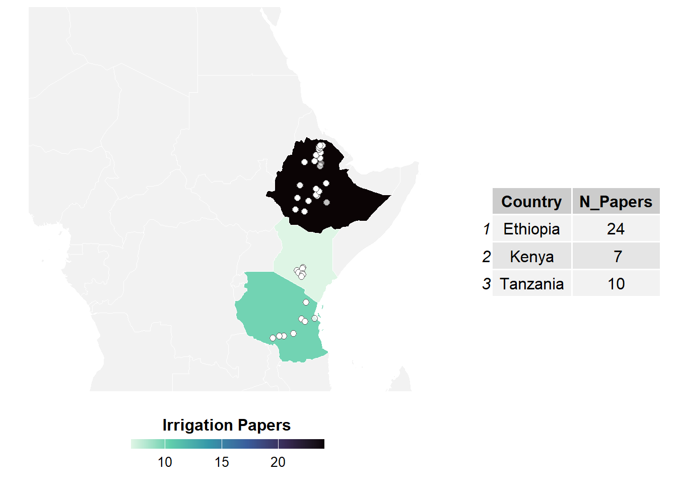
1.5 Exploring geographic locations of studies available

We collected country, site name paraphrased from study, and spatial coordinates when given. Location’s coordinates were verified in Google Maps, as they were often inaccurately reported. Enumerators also recorded a measure of spatial uncertainty. When authors reported decimal degrees and there was no correction required to the co-ordinates, then uncertainty was measured in terms of the value’s precision. When the location was estimated using Google Maps, the spatial uncertainty value was measured in terms of the precision of the site location description (e.g., a single farm or region) and the enumerator’s visual interpretation of land use at and near the coordinates. Observation’s geographic coordinates were collected to facilitate linking the data compiled in ERA to external databases, for example related to climatic and environmental factors not necessarily reported in the original study.

Code

# ---- Data prep ----
# Ensure coordinates are numeric
irrigation_data <- irrigation_data %>%
  mutate(
    Latitude = as.numeric(Latitude),
    Longitude = as.numeric(Longitude)
  ) %>%
  filter(!is.na(Latitude) & !is.na(Longitude))

# Count the number of papers per country
paper_counts <- irrigation_data %>%
  group_by(Country) %>%
  summarise(N_Papers = n_distinct(Code), .groups = "drop")

# Load only African countries and fix naming
world <- ne_countries(scale = "medium", continent = "Africa", returnclass = "sf") %>%
  mutate(admin = if_else(admin == "United Republic of Tanzania", "Tanzania", admin))

# Transform CRS
world <- st_transform(world, crs = 4326)

# Convert points to sf object
sites_sf <- st_as_sf(irrigation_data, coords = c("Longitude", "Latitude"), crs = 4326, remove = FALSE)

# Prepare map data
map_data <- world %>%
  dplyr::select(admin, geometry) %>%
  rename(Country = admin) %>%
  left_join(paper_counts, by = "Country")

# ---- Create map ----
map <- ggplot() +
  geom_sf(data = map_data, aes(fill = N_Papers), color = "white") +
  geom_point(data = sites_sf, aes(x = Longitude, y = Latitude), 
             shape = 21, color = "black", fill = "white", size = 2, alpha = 0.5) +
  scale_fill_viridis_c(
    option = "mako",
    direction = -1,
    na.value = "gray95"
  ) +
  labs(fill = "Irrigation Papers") +
  theme_minimal() +
  theme(
    legend.position = "bottom",
    legend.direction = "horizontal",
    legend.title = element_text(size = 12, face = "bold"),
    legend.text = element_text(size = 10),
    axis.text = element_blank(),
    axis.ticks = element_blank(),
    axis.title = element_blank(),
    panel.grid = element_blank()
  ) +
  guides(fill = guide_colorbar(
    barwidth = 10, barheight = 0.5, title.position = "top", title.hjust = 0.5
  )) +
  coord_sf(xlim = c(5, 52), ylim = c(-15, 30), expand = FALSE)  # Zoom to East Africa

# ---- Create static table grob ----
table_grob <- tableGrob(head(paper_counts, 20))  # Show top 20 countries

# ---- Plot map and table side by side ----
grid.arrange(map, table_grob, ncol = 2, widths = c(2, 1))

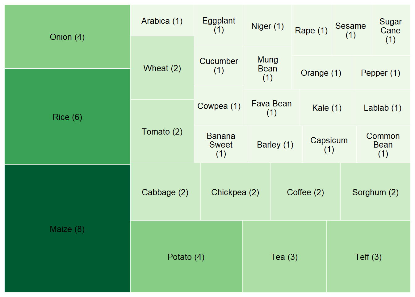
1.6 Exploring the products of studies available

The Product.Subtype column in the ERA.Compiled_ag dataset contains the specific crop types examined in each study (e.g., "Maize", "Rice", "Wheat").

To accurately count how many unique studies (identified by Code) examined each crop, the following code processes and summarizes the data.

The figure below displays the distribution of crop categories in the dataset. It highlights the relative focus of studies across different crop types.

The largest category by far is Cereals, indicating that most studies in ERA are focused on cereal crops such as maize, wheat, rice, and sorghum.
This is followed by Legumes, Starchy Staples, and Vegetables, which also appear frequently in the dataset.
Categories such as Fodders, Cash Crops, and Fruits are represented to a lesser extent.

Each tile represents a crop category, and its size reflects the number of unique studies (Code) that included at least one crop from that category. The number in parentheses shows the count of studies for that group.

Code

prod_counts <- irrigation_data %>%
  separate_rows(Product.Simple, sep = "-") %>% 
  group_by(Product.Simple) %>%
  summarise(Count = n_distinct(Code), .groups = "drop") %>%
  mutate(label = paste0(Product.Simple, " (", Count, ")"))


tree_plot<- ggplot(prod_counts, aes(area = Count, fill = Count, label = label)) +
  geom_treemap(color = "white") +
  geom_treemap_text(
    colour = "black",
    place = "centre",
    grow = FALSE,       # Disable growing to avoid oversized text
    reflow = TRUE,
    size = 10            # Adjust this value to control the actual text size
  ) +
  scale_fill_distiller(palette = "Greens", direction = 1, guide = "none") +
  theme_minimal() +
  theme(
    plot.title = element_text(size = 14, face = "bold"),
    legend.position = "none"
  )
tree_plot

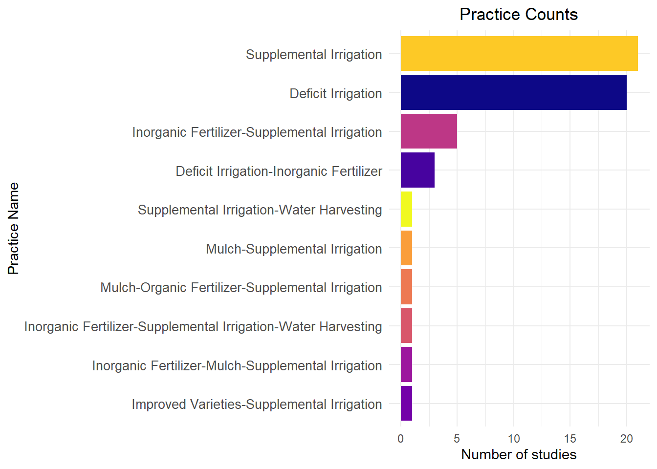
1.7 Exploring the agronomic practices within studies available

The following analysis explores the types of agronomic practices-referred to as “Themes” in the dataset.

Each study in ERA may be associated with multiple practices—for example, a study might examine both Soil Management and Nutrient Management.
For example, the theme ‘Soil Management’ include practices like green manure, crop residue, pH control, tillage, improved fallows. ‘Nutrient Management’ includes organic and inorganic fertilizer. This can be found in the practices within the mastercodes

Code


# Calculate counts
ag_counts <- irrigation_data %>%
  group_by(PrName) %>%
  summarise(Count = n_distinct(Code), .groups = "drop") %>%
  mutate(label = paste0(PrName, " (", Count, ")"))

# Bar plot
bar_plot <- ggplot(ag_counts, aes(x = reorder(PrName, Count), y = Count, fill = PrName)) +
  geom_col(show.legend = FALSE) +
  coord_flip() +
  labs(
    title = "Practice Counts",
    x = "Practice Name",
    y = "Number of studies"
  ) +
  scale_fill_viridis_d(option = "plasma") +
  theme_minimal() +
  theme(
    axis.text.y = element_text(size = 10),
    plot.title = element_text(hjust = 0.5)
  )

bar_plot

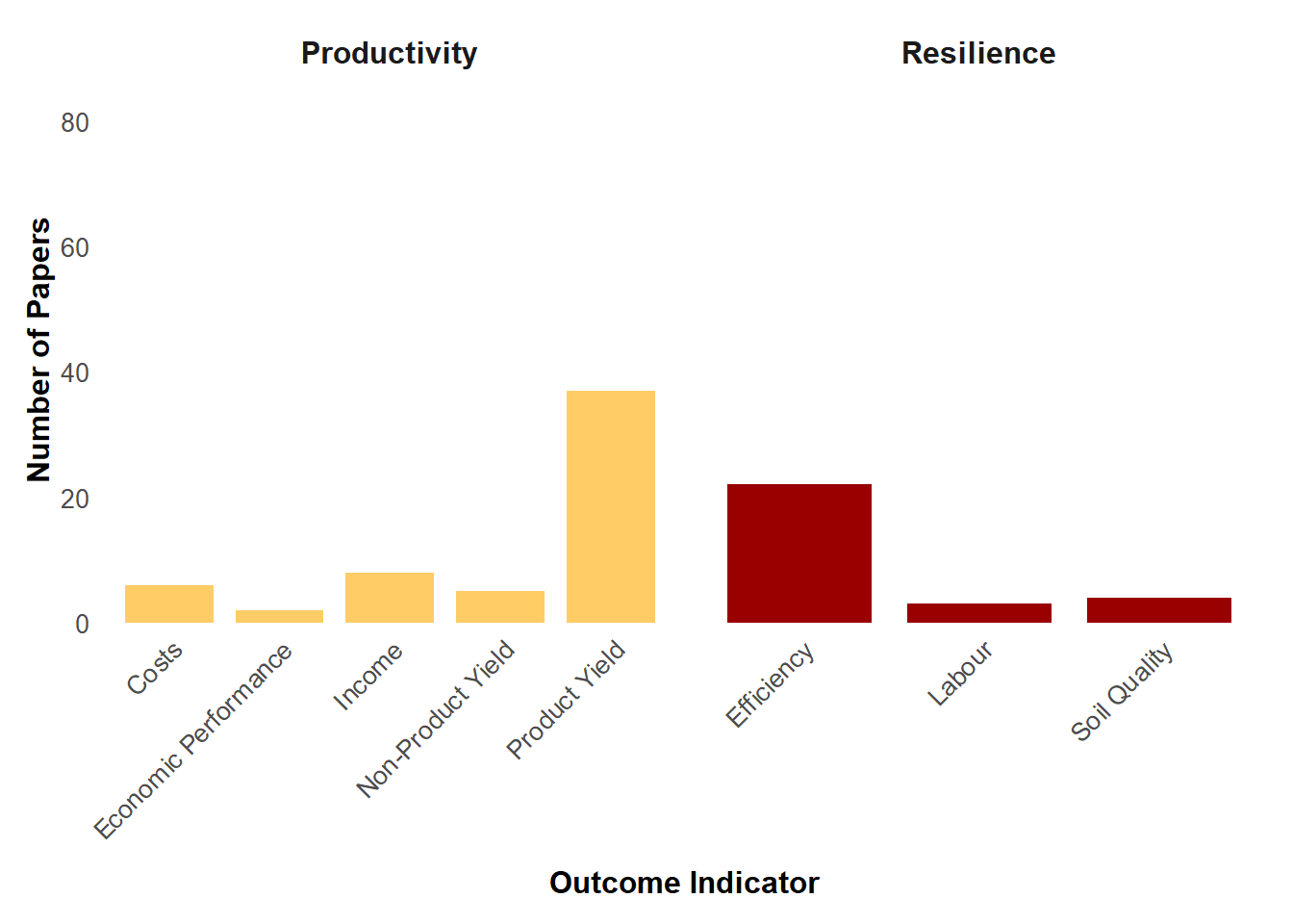
1.8 Exploring the outcomes reported within studies available

The ERA dataset tracks outcomes of agronomic interventions across several broad categories—called Pillars—such as productivity, environmental impact, and more. Each pillar includes more specific indicators like yield, GHG emissions, soil organic carbon, and others.

Code

# Aggregate data by pillar and indicator
out_counts <- irrigation_data %>%
  mutate(Out.Pillar = trimws(as.character(Out.Pillar))) %>%
  filter(Out.Pillar != "", !is.na(Out.Pillar), !is.na(Out.Ind)) %>%
  group_by(Out.Pillar, Out.Ind) %>%
  summarise(Num_Papers = n_distinct(Code), .groups = "drop") %>%
  rename(Pillar = Out.Pillar, Indicator = Out.Ind)


# Sort indicators within each pillar
out_counts <- out_counts %>%
  arrange(Pillar, Indicator) %>%
  mutate(
    Indicator = factor(Indicator, levels = unique(Indicator)),
    Pillar = factor(Pillar, levels = c("Productivity", "Resilience"))
  )

# Optional: define pillar colors
pillar_colors <- c(
  "Productivity" = "#FFCC66",
  "Resilience" = "#990000"
)

out_counts <- out_counts %>%
  filter(
    !is.na(Pillar), Pillar != "",
    !is.na(Indicator), Indicator != ""
  )


# Plot
bar_plot <- ggplot(out_counts, aes(
  x = Indicator, y = Num_Papers, fill = Pillar
)) +
  geom_col(width = 0.8) +
  labs(
    y = "Number of Papers",
    x = "Outcome Indicator"
  ) +
  scale_fill_manual(values = pillar_colors, na.value = "gray70") +
  scale_y_continuous(
    limits = c(0, max(out_counts$Num_Papers) + 50),
    expand = c(0, 0)
  ) +
  facet_wrap(~Pillar, scales = "free_x", nrow = 1) +
  theme_minimal() +
  theme(
    axis.text.x = element_text(size = 10, angle = 45, hjust = 1),
    axis.text.y = element_text(size = 10),
    axis.title.x = element_text(size = 12, face = "bold", margin = margin(t = 10)),
    axis.title.y = element_text(size = 12, face = "bold"),
    legend.position = "none",
    panel.grid.major = element_blank(),
    panel.grid.minor = element_blank(),
    strip.text = element_text(size = 12, face = "bold"),
    plot.margin = margin(10, 10, 10, 10)
  )

# Show plot
bar_plot