Introduction to ERA

This vignette will guide you through the agronomy data available within the Evidence for Resilient Agriculture (ERA). The data set serves as a critical resource for understanding agricultural outcome trade-offs and synergies between yield, economic performance, sustianability indicators, and climate resilience. It focuses on peer-reviewed data from experimental or observation agriculture systems. If you are interested in livestock please see ERL.

We will cover the following:

What is ERA:

• Introduction – What ERA is, where it comes from, and what it contains
  
• Extraction template – How the ERA Excel template structures studies and practices
  
• Understanding the ERA data model – Structure and content of the raw data tables
  
• Comparisons table – A simplified format for quick meta-analysis
  
• Controlled vocabulary – ERA’s structured codes for harmonized interpretation
  
• Spatial locations and uncertainty – How geographic context is handled

Downloading the data:

• Downloading the ERA.Compiled comparisons table
  
• Downloading the data model tables
  
• Downloading the controlled vocabulary
  
• Viewing the data catalog

Exploring the data:

• Sub-setting the data to agronomy
  
• Exploring geographic locations of studies
  
• Exploring crop types (products) in the data
  
• Exploring agronomic practices used in the studies
  
• Exploring the outcomes reported

Worked Example:

• Analyzing maize yield response using the comparisons table

Additional tools and learning:

• Vignettes from the ERAg package – Further worked examples and methods

1 What is ERA?

1.1 Introduction

The Evidence for Resilient Agriculture (ERA) initiative was launched in 2012 to address the need for a robust evidence base on how agricultural practices perform under different conditions. Originally developed to evaluate the outcomes of Climate-Smart Agriculture (CSA), ERA has since evolved to include a wide range of technologies and practices relevant to agroecology, regenerative agriculture, ecosystem-based adaptation, and nature-based solutions.

ERA provides a large, structured meta-dataset of agricultural experiments, harmonized using a common data model and controlled vocabulary. The current version of the dataset (version = era_compiled-v1.0-mh_2025-03-19.2-sc_2025_01_30.1-ie_2025_03_19.1-2025-03-28.1) includes 193835 observations from 2902 peer-reviewed agricultural studies conducted in Africa between 1934 and 2022. These observations cover more than 451 unique combinations of practices, and assess their effects on over 97 outcome indicators, including yield, soil health, and emissions.

Experiments were identified through systematic searches in Web of Science and Scopus and were screened against predefined criteria: geographic location, technology and outcome relevance, inclusion of both conventional and alternative treatments, and availability of primary data. The extracted data are structured using a detailed Excel-based template, enabling flexible and precise representation of treatments, outcomes, experimental design, and context.

A derived product, the ERA.Compiled table, simplifies the dataset into treatment-control comparisons, making it easier to analyze the effects of agricultural interventions. While the compiled table is ideal for quick analysis, it remains linked to the full data model, allowing users to retrieve detailed metadata and contextual information where needed.

1.2 Extraction template

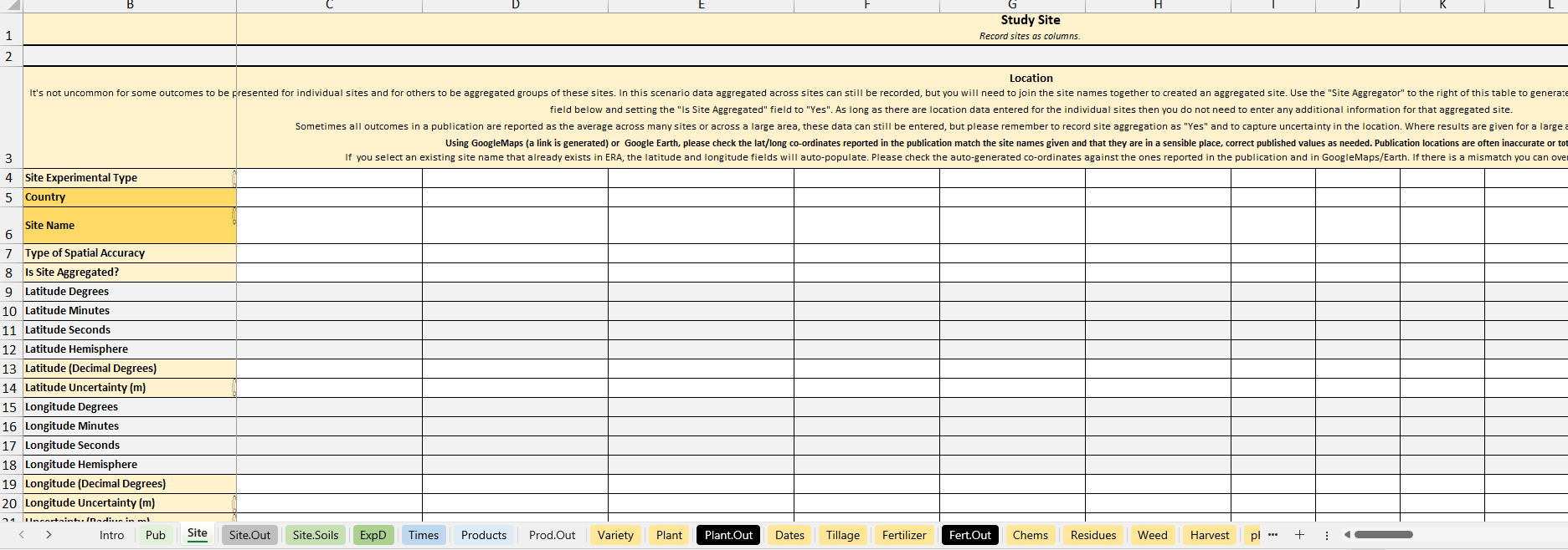
Over the years of ERA, several versions of the extraction template have been developed. However, the most widely used and thoroughly tested version is the Excel macro-enabled workbook. In this format, each study is documented in a separate Excel file, with individual tabs dedicated to different components of the study—such as site information, soil characteristics, management practices, and outcomes. The work book contains the following sections:

1. Pub = Publication: capture bibliographic data about an experiment here.

2. Site & Site Soils = captures information about experimental sites, any detailed information about soil variables should be captured in Site.Soils

3. ExpD = Experimental design, captures information about the number of study replicates, plot sizes, etc.

4. Practices (pale yellow tabs) = These tabs collect information about the agricultural management practices used in an experiment. Within tabs you can record base practices which apply to all treatments (e.g. 50kg of 60-30-30 NPK was applied to all treatments) or experimental practices that different between treatments (e.g. one treatment used straw mulch and another did not). Each set of experimental practices within a practice tab creates named building blocks that you will combine in the Make.Trt tab to create treatments. Base practices you do not need to consider again once they are entered in the practice tabs, they also do not require naming as the spreadsheet should autopopulate the name field with “base”.

   Many practice tabs will require you to select and name a practice method that relates to a code in ERA practice definitions, this part of the data entry is critical. After you have chosen a method and named a practice you can often scroll down to tables that can collect more detail information about how the practice was implemented. There are also notes sections where you can copy paste important experimental information that you do no think the workbook captures well. Each tab is a theme that represents a set of related practices:

   • Chems = Chemical applications (applications of herbicides, fungicides, insecticides, etc.)

   • Harvest = Harvest methods & timing Irrigat = Irrigation methods & application rates

   • Mulch = Materials that are not from crops in the experimental plot (record these in the residues tab) applied to the surface of the plot as a mulch. Records the type of mulch & application details . Does not include compost or manures (use the nutrients tab).

   • Nutrients = Inputs/fertilizers added to a plot designed to improve/increase/provide nutrients for crop growth. Nutrients can include inorganic fertilizers, compost, manure, micronutrients, biochar, biofertilizers, biosolids and other organic amendments. Records the type of fertilizer & application details.

   • Comp = Composition of organic mulch or nutrient materials.

   • pH = Materials & application rates of materials used for amendment of soil pH (e.g. liming).

   • Plant = Planting methods & timing Residues = Fate of crop residues & compositional details.

   • Tillage = Tillage method(s) used & details of tillage operations.

   • Variety = Crop varieties used & information on their basic traits.

   • WaterHarvest = Water harvesting methods (e.g., planting basins, terraces, tied ridges, zai pits, etc.).

   • Weed = Physical (not chemical) weeding events (typically hand weeding).

5. Make.Trt = Create & name treatments by combining the experimental practices entered in the practice tabs.

6. Intercropping = Combine the crop specific treatments created in the Make.Trt tab to describe intercropping systems.

7. Time.Seq (Rotations) = Create temporal sequences of treatments and/or intercrops to reflect, for example, crop rotations or fallows.

8. EU&Out = Experimental Unit & Outcomes: Choose the experimental units (typically crop or animal commodities) and experimental outcomes for which data are presented.

9. Times = Select the cropping seasons or years for which data are presented.

10. EnterData = Captures values and associated errors for the experimental treatments, products, outcomes and times specified in the previous tabs. Do not start data entry until you’ve completed all the previous tabs.

The link to this extraction template can be found here: https://github.com/CIAT/ERA_dev/blob/main/data_entry/industrious_elephant_2023/excel_data_extraction_template/V2.0.28%20-%20Industrious%20Elephant.xlsm

Click on the image below to watch a short tutorial on the extraction template

Watch on YouTube

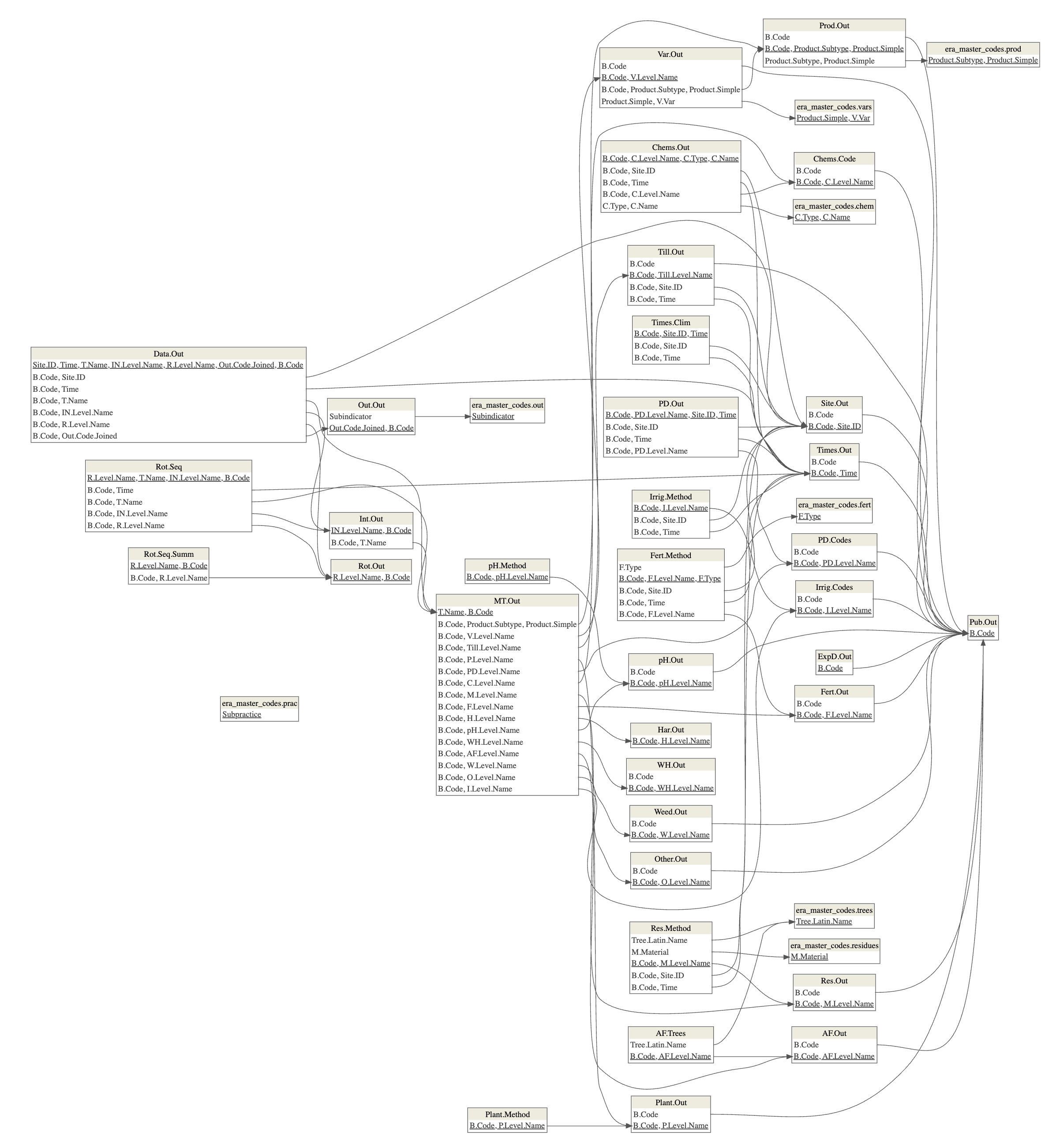
1.3 Data model (raw data)

Each of the tables within the front end of the excel feeds are imported using R to generate tables that form a data model. These tables provide you with detailed information from each study, e.g fertilizer applied, timing of fertilizer and so on.

The main tables are:

• Pub.Out : Publication information, DOIs, ERA template version and project.
• Site.Out,Soils.Out : Location, coordinates, location uncertainty radius, site/location type, site soils.
• ExpD.Out : Experimental design.
• Times.Out : Measurement periods for which experimental results are reported (typically growing seasons).
• Times.Clim : Climate information for locations x measurement periods recorded in Times.Out (e.g. rainfall for particular growing season).
• Prod.Out : Crop or animal commodity.
• Var.Out : Variety and any usual associated information reported.
• Till.Out : Tillage management.
• Plant.Out,Plant.Method : Planting information (density, arrangement, thinning, etc.).
• PD.Codes,PD.Out: Management practices that relate to improved timing of planting activities and information on planting and harvest dates.
• Fert.Out,Fert.Method,Fert.Comp: Detailed fertilizer management and composition of organic fertilizers.
• Chems.Code,Chems.Out,Chems.AI : Chemicals applications (pesticides, veterinary medicines, and chemicals that do not fit the definition of a fertilizer).
• Res.Out,Res.Method,Res.Comp : Information on mulching or crop residue management.
• Har.Out :Improved harvesting.
• pH.Out : pH management.
• WH.Out : Water harvesting practices.
• Irrig.Codes,Irrig.Methods: Irrigation management practices and applications.
• AF.Out,AF.Trees: Agroforestry management and tree species and density.
  
• Int.Out : Intercropping management.
• Rot.Out``Rot.Seq,Rot.Seq.Summ : Crop rotations or other temporal sequence of managment activities.
• Out.Out,Out.Econ : The Outcomes reported in the experiment and any additional context required for understanding them (e.g. discount rate and time period for economic outcomes).
• Data.Out : Reported values and errors for combinations of outcome, commodity, management (treatment, intercrop, and/or rotation), location, and time (measurement period).

The data model also makes use of a large controlled vocabulary (the master codes), which is described later in this document. We aspire to develop the controlled vocabulary into an ontology for agricultural meta-analysis. A beta-version for livestock can be found here

More detailed documentation of the ERA agronomy data model is available here.

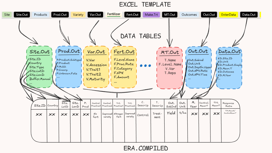
1.4 Comparisons table

In an attempt to make ERA data easily usable, we provide a table of control vs. treatment comparisons (ERA.Compiled). This is a flat excel file that pulls only essential fields from each data table table to create rows of treatment versus control. The table does not include detailed descriptions of management practices, but it can be connected back to the ERA data model if specific management information is required.

It should be noted that more studies are available in the comparisons table than the data model. This is because the earliest iteration of ERA used this flat template (ERA.Compiled) to extract data. We do not have the resources to convert all extractions to the data model.

Below is a simple conceptional framework of how ERA.Compiled is generated from the data tables.

1.5 Controlled vocabulary

ERA uses a structured controlled vocabulary to ensure consistency and harmonization across thousands of experimental observations. This vocabulary underpins the data model and comparison table by standardizing the names and attributes of practices, outcomes, and management components. It is compiled into an Excel workbook (era_master_sheet.xlsx) and is essential for:

• Defining practice types (e.g., fertilizer, tillage, variety)
• Classifying input materials (e.g., specific fertilizer types or tree species)
• Linking outcomes to clear definitions and measurement units
• Supporting interoperability and reproducibility in meta-analyses

The vocabulary is organized into multiple sheets, each corresponding to a different concept area, including:

• era_fields_v1: data catalog for comparisons table (ERA.Compiled)
• era_fields_v2: data catalog for data model (work in progress)
• prod: commodity types and product subtypes
• fert: fertilizer types
• chem: chemical types (e.g. pesticides)
• chem.comm: commercial chemical names
• chem.ai: active ingredients
• trees: agroforestry tree species
• vars: crop varieties and associated traits
• out: outcome subindicators
• prac: subpractices and method types (e.g. planting method, tillage type)
• residues: residue management material types
• lookup_levels: controlled values for data entry lookups
• site_list: standardized locations for agricultural experiment or demonstration sites
• unit_harmonization: harmonization table to standardize unit naming

These vocabularies are linked to the main ERA data tables via foreign key relationships in the dm data model. For example, the Fert.Method table contains a column F.Type, which links to the fert sheet of the master codes. This structure ensures that the dataset can be queried and interpreted accurately at scale.

A future goal is to evolve this vocabulary into a full ontology for agricultural meta-analysis, aligning it with existing semantic web and ontology standards. A beta-version of the livestock ontology is already underway.

The most up-to-date version of the vocabulary can be accessed here:

ERA Master Vocabulary (Excel)

1.6 Spatial locations and uncertainty

ERA captures the geographic context of each experiment to support spatial analyses and linkages to climate, soil, and other environmental datasets. Coordinates are reported in decimal degrees (WGS84; EPSG:4326).

Each observation includes a spatial uncertainty estimate, recorded in the field Buffer (in meters), which represents the radius around the point location within which the true experimental site is likely to fall. This allows users to account for geolocation confidence when integrating with gridded datasets.

Spatial metadata is included in the Site.Out table of the data model, the comparisons table and in a reference sheet called era_master_codes$site_list within the controlled vocabulary workbook. Spatial fields include:

• Standardized site name (Site.ID): Unique names used to identify experimental sites across studies. These are harmonized for locations that appear in multiple studies under varying names. When multiple sites are aggregated in a single observation, their names are joined with “..” (e.g., “Mbinga..Nkhata Bay”).
• Latitude and Longitude: Verified coordinates in WGS 1984 (EPSG:4326), either reported by authors or manually geolocated by curators.
• Uncertainty radius (Buffer): Numeric value in meters, reflecting spatial precision of the location (e.g., village, district, coordinates with varying decimal precision).
• Site type (Site.Type): Describes whether the site is an on-farm trial, experimental station, or another type of location.
• Site key (Site.Key): A standardized code combining the latitude (to 4 decimal places), longitude (to 4 decimal places), and Buffer value. This uniquely identifies the geospatial footprint of a site across the entire dataset. For example, “06.7170 -1.5333 B500” refers to a site at latitude 6.7170, longitude –1.5333, with a 500m uncertainty radius. This field is used to cluster spatially similar sites and support spatial matching.

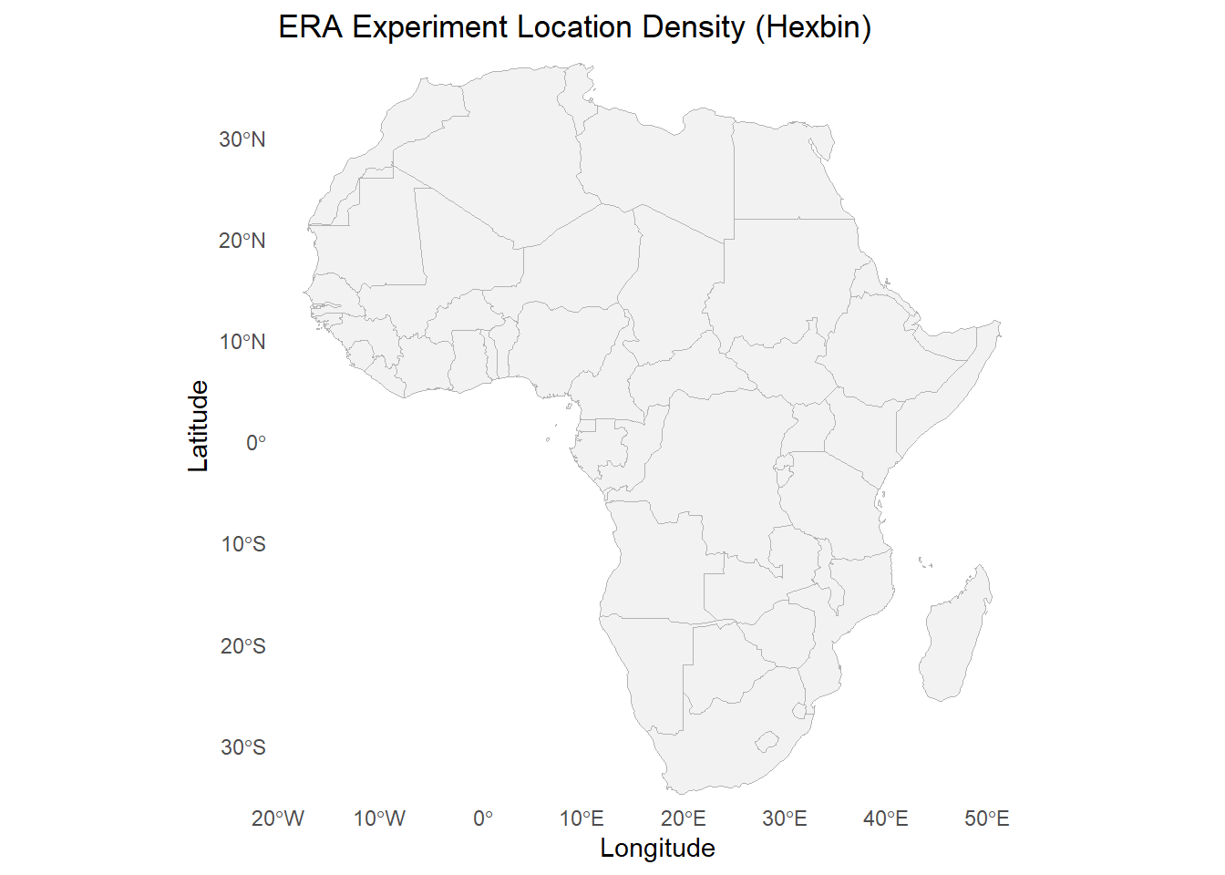
R code:

library(ggplot2)
library(data.table)
library(rnaturalearth)
library(rnaturalearthdata)
library(sf)
library(viridis)

# 1. Subset ERA.Compiled to unique study x lat/lon combinations (non-missing)
site_locs <- ERA_Compiled[!is.na(Latitude) & !is.na(Longitude), .(Latitude, Longitude, Buffer,Code)]
site_locs <- unique(site_locs)

# 2. Load Africa country shapes as sf object
africa <- ne_countries(continent = "Africa", scale = "medium", returnclass = "sf")

# 3. Plot with hex bins
ggplot() +
  geom_sf(data = africa, fill = "grey95", color = "grey70", linewidth = 0.3) +
  geom_hex(
    data = site_locs,
    aes(x = Longitude, y = Latitude),
    bins = 80,                   
    alpha = 0.8
  ) +
  scale_fill_viridis_c(
    option = "turbo",
    direction = 1,
    na.value = "transparent"
  ) +
  coord_sf(xlim = c(-20, 55), ylim = c(-35, 38), expand = FALSE) +
  theme_minimal() +
  labs(
    title = "ERA Experiment Location Density (Hexbin)",
    x = "Longitude",
    y = "Latitude"
  ) +
  theme(
    panel.grid = element_blank()
  )

python code:

# Python equivalent code:

import pandas as pd
import geopandas as gpd
import matplotlib.pyplot as plt
import matplotlib as mpl

# 1. Subset ERA_Compiled to unique study x lat/lon combinations (non-missing)
site_locs = (
    ERA_Compiled
    .dropna(subset=['Latitude', 'Longitude'])
    [['Latitude', 'Longitude', 'Buffer', 'Code']]
    .drop_duplicates()
)

# 2. Load Africa country shapes as a GeoDataFrame
world = gpd.read_file(gpd.datasets.get_path('naturalearth_lowres'))
africa = world[world['continent'] == "Africa"]

# 3. Plot with hex bins
fig, ax = plt.subplots(figsize=(10, 8))

# Plot Africa boundaries with a light grey fill and slightly darker borders
africa.plot(ax=ax, color="grey95", edgecolor="grey70", linewidth=0.3)

# Create a hexbin plot for site locations with gridsize=80 and alpha transparency
hb = ax.hexbin(
    site_locs['Longitude'], 
    site_locs['Latitude'],
    gridsize=80,
    cmap=mpl.cm.get_cmap("turbo"),
    alpha=0.8
)

# Add a colorbar to indicate the count scale
cb = fig.colorbar(hb, ax=ax)
cb.set_label('Count')

# Set coordinate limits to match the original R plot
ax.set_xlim(-20, 55)
ax.set_ylim(-35, 38)

# Add title and axis labels
ax.set_title("ERA Experiment Location Density (Hexbin)", fontsize=14)
ax.set_xlabel("Longitude", fontsize=12)
ax.set_ylabel("Latitude", fontsize=12)

# Remove grid lines to mimic a minimal theme
ax.grid(False)

plt.show()

The site_list contains standardized locations for agricultural research or demonstration facilities to help standardize and harmonize location reporting during data extraction and compilation.

For all locations—whether reported as coordinates by the original authors or estimated—ERA applies a rigorous two-stage human validation process. This includes:
- Checking that the coordinates correspond to agriculturally plausible areas (e.g., not in oceans, mountains, or cities). - Ensuring consistency with the site description in the publication. - Correcting erroneous coordinates (e.g., swapped lat/lon, misplaced decimals). - Geolocating sites where no coordinates were given, based on textual descriptions. - Assigning an appropriate uncertainty radius depending on location specificity (e.g., “county” vs “village” vs “research station”).

This spatial verification process ensures ERA’s location data is suitable for integration with remote sensing, climate, and other geospatial datasets.

In some cases, a single observation may represent results aggregated across multiple spatial locations. These cases are identified in the Site.ID field using a .. delimiter (e.g., "Kiberashi..Mbinga..Nkhata Bay"). Each component site is described individually in the site_list, including its coordinates and uncertainty radius. For aggregated sites, ERA computes a centroid of all included sites, and the overall spatial uncertainty (Buffer) is calculated as the distance from this centroid to the edge of the furthest site’s uncertainty buffer. This ensures that even spatially aggregated results are represented with an appropriate spatial footprint.

Spatial locations connect ERA to wider geospatial information, find out more in the Guide to Climate and Soil Data in ERA.

2 Download the data

Data is openly available for download from the S3 Bucket s3://digital-atlas/era/data/.

2.1 Download controlled vocabulary

This section downloads and imports the ERA controlled vocabulary, which standardizes the naming of practices, products, and outcomes across studies. Both R and Python code examples are provided.

R code:

# Download the era master vocab ######
era_vocab_url <- "https://github.com/peetmate/era_codes/raw/main/era_master_sheet.xlsx"
era_vocab_local <- file.path(dl_dir, basename(era_vocab_url))
if(!file.exists(era_vocab_local)|update_vocab){
  download.file(era_vocab_url, era_vocab_local, mode = "wb")  # Download and write in binary mode
}
  
# Import the vocab
sheet_names <- readxl::excel_sheets(era_vocab_local)
sheet_names <- sheet_names[!grepl("sheet|Sheet", sheet_names)]

# Read each sheet into a list named era_master_codes
era_master_codes <- sapply(
  sheet_names,
  FUN = function(x) {
    data.table::data.table(readxl::read_excel(era_vocab_local, sheet = x))
  },
  USE.NAMES = TRUE
)

python code:

# Note: This is a GPT-generated Python translation and requires validation.
import os
import requests
import pandas as pd

# Define download directory
dl_dir = "era_master_codes"
os.makedirs(dl_dir, exist_ok=True)

# Define URL and local path
era_vocab_url = "https://github.com/peetmate/era_codes/raw/main/era_master_sheet.xlsx"
era_vocab_local = os.path.join(dl_dir, os.path.basename(era_vocab_url))

# Download the file if it doesn't already exist
if not os.path.exists(era_vocab_local):
    response = requests.get(era_vocab_url)
    with open(era_vocab_local, "wb") as f:
        f.write(response.content)

# Read all sheets except those with "sheet" in the name
xls = pd.ExcelFile(era_vocab_local)
sheet_names = [s for s in xls.sheet_names if "sheet" not in s.lower()]

# Load each sheet into a dictionary
era_master_codes = {
    sheet: xls.parse(sheet) for sheet in sheet_names
}

How you can explore descriptions of major ERA concepts (Practices, Outcomes, Products):

R code:

practices<- era_master_codes$prac[,.(Code,Theme,Practice,Subpractice,Definition)]

DT::datatable(
  practices,
  options = list(
    scrollY = "400px",scrollX = TRUE,pageLength = 50,fixedHeader = FALSE 
  ),
    caption = htmltools::tags$caption(
    style = "caption-side: top; text-align: left; font-weight: bold; font-size: 1.1em;",
    "management practice definitions"
    ),
    class = "nowrap"
)

R code:

outcomes<- era_master_codes$out[,.(Code,Pillar,Pillar.Code,Subpillar,Indicator,Subindicator,Definition)]
DT::datatable(
  outcomes,
  options = list(
    scrollY = "400px",scrollX = TRUE,pageLength = 20,fixedHeader = FALSE,
    columnDefs = list(
      list(width = '100px', targets = which(names(outcomes) == "Definition") - 1)
    )
  ),
  class = "nowrap",
  caption = htmltools::tags$caption(
    style = "caption-side: top; text-align: left; font-weight: bold; font-size: 1.1em;",
    "outcome definitions"
    )
)

R code:

products<- era_master_codes$prod[,.(EU,Product.Type,Product.Subtype,Product,Product.Simple,Component,Latin.Name)]
DT::datatable(
  products,
  options = list(
    scrollY = "400px",scrollX = TRUE,pageLength = 50,fixedHeader = FALSE 

  ),
 caption = htmltools::tags$caption(
    style = "caption-side: top; text-align: left; font-weight: bold; font-size: 1.1em;",
    "products (a.k.a. experimental units)"
    )
)

python code:

import pandas as pd
from IPython.display import display

# Extract tables from the loaded Excel sheets
practices = era_master_codes["prac"]
outcomes = era_master_codes["out"]
products = era_master_codes["prod"]

# Display tables with scrollable options in JupyterLab/Notebook
with pd.option_context('display.max_rows', 20, 'display.max_columns', None):
    display(practices.style.set_table_attributes("style='display:inline; float:left; margin-right:20px;'"))
    display(outcomes.style.set_table_attributes("style='display:inline; float:left; margin-right:20px;'"))
    display(products.style.set_table_attributes("style='display:inline; float:left; margin-right:20px;'"))

2.2 Download data model

This section connects to the public S3 bucket, identifies the latest agronomic ERA data set, downloads it locally, and loads it into memory.

R code:

# Create an S3 filesystem handle
s3 <- s3fs::S3FileSystem$new(anonymous = TRUE)
era_s3 <- "s3://digital-atlas/era"

# List files in the s3 bucket
all_files <- s3$dir_ls(file.path(era_s3, "data"))

# Filter for the "agronomic" RData file, selecting the most recent version
target_file <- tail(
  grep(".RData", grep("agronomic", all_files, value = TRUE), value = TRUE),
  1
)

# Define a local path for saving the downloaded file
save_path <- file.path(dl_dir, basename(target_file))

# Download the file if it does not exist already
if (!file.exists(save_path)) {
  s3$file_download(target_file, save_path, overwrite = TRUE)
}

# Load the agronomy data using the miceadds package
agronomic_data <- miceadds::load.Rdata2(
  file = basename(save_path),
  path = dirname(save_path)
)

python code:

# Note: This is a GPT-generated Python translation and requires validation.
import os
import s3fs
import re

# Define download directory
dl_dir = "downloaded_data"
os.makedirs(dl_dir, exist_ok=True)

# Set up anonymous S3 filesystem
s3 = s3fs.S3FileSystem(anon=True)
era_s3 = "digital-atlas/era/data"

# List files in the S3 bucket
all_files = s3.ls(era_s3)

# Filter for latest agronomic .RData file
agronomic_files = [f for f in all_files if "agronomic" in f and f.endswith(".RData")]
target_file = sorted(agronomic_files)[-1] if agronomic_files else None

# Define local save path
save_path = os.path.join(dl_dir, os.path.basename(target_file))

# Download file if not already present
if not os.path.exists(save_path):
    with s3.open(target_file, 'rb') as src, open(save_path, 'wb') as dst:
        dst.write(src.read())

# Note: RData file loading requires R. Consider using `rpy2` if needed.

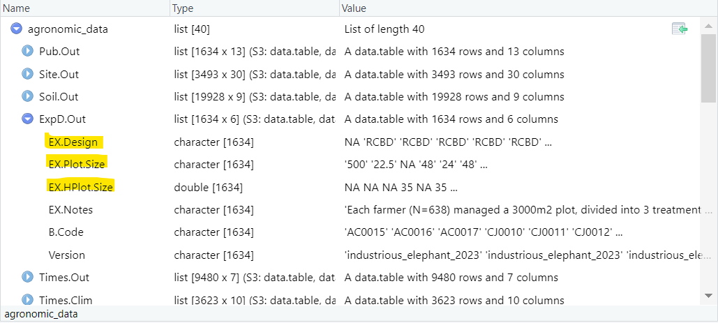
Once the data is downloaded, it will appear as the screenshot below.

Each of the tables can be extracted individual and combined with one another based on a common piece of information. For example, the B.Code, which is present in each tab, can be used to match information from one particular paper across all these tables.

To get a better understanding of what the fields in the data model are you can view data a catalog by running the following code:

R code:

# Access era_fields from era_master_codes
era_fields <- era_master_codes$era_fields_v2

# Filter to the version relevant to the agronomy data model
era_fields<-era_fields[industrious_elephant_2023==T,.(Table,Field,Display_Name,Field_Description,Data_Type)]

names(era_fields)
#> [1] "Table"             "Field"             "Display_Name"     
#> [4] "Field_Description" "Data_Type"

python code:

# Access and filter the era_fields_v2 sheet
era_fields_df = era_master_codes["era_fields_v2"]

# Filter to the version relevant to the agronomy data model
filtered_fields = era_fields_df[era_fields_df["industrious_elephant_2023"] == True]

# Select specific columns
era_fields = filtered_fields[["Table", "Field", "Display_Name", "Field_Description", "Data_Type"]]

# Show column names
print(era_fields.columns.tolist())

Note the data catalog era_master_codes$era_fields_v2 is a work in progress, we are currently revising it and it should be completed by May 2025.

See our agronomy data model page for more information how the data tables are connected.

2.3 Download comparisons table

This section retrieves the most recent version of the ERA.Compiled comparisons table from the ERA S3 bucket, saves it locally, and loads it for use.

R code:

s3 <- s3fs::S3FileSystem$new(anonymous = TRUE)
era_s3 <- "s3://digital-atlas/era"

# List files in the s3 bucket
all_files <- s3$dir_ls(file.path(era_s3, "data"))

# Filter for the "agronomic" RData file, selecting the most recent version
# Filter for the correct compiled comparison CSV
(target_file_compiled <- all_files[
  grepl("era_compiled.*mh.*csv$", all_files, ignore.case = TRUE) &
    !grepl("econ", all_files, ignore.case = TRUE) 
] |> tail(1))
#> [1] "s3://digital-atlas/era/data/era_compiled-v1.0-mh_2025-03-19.2-sc_2025_01_30.1-ie_2025_03_19.1-2025-03-28.1.csv"

# The file will start era_compiled, should not contain econ and the most recent version will have the most recent
# date at the end of the file name.

# Define a local path for saving the downloaded file
save_path <- file.path(dl_dir, basename(target_file_compiled))

# Download the file if it does not exist already
if (!file.exists(save_path)) {
  s3$file_download(target_file_compiled, save_path, overwrite = TRUE)
}

# Load the data
ERA_Compiled <- fread(save_path)

python code:

import os
import s3fs
import pandas as pd

# Set up S3 access
fs = s3fs.S3FileSystem(anon=True)
era_s3 = "digital-atlas/era/data"
dl_dir = "era_master_codes"
os.makedirs(dl_dir, exist_ok=True)

# List files in the S3 directory
all_files = fs.ls(era_s3)

# Filter for most recent compiled CSV (excluding "econ")
compiled_files = sorted([
    f for f in all_files
    if "era_compiled" in f.lower()
    and "mh" in f.lower()
    and f.lower().endswith(".csv")
    and "econ" not in f.lower()
])

# Select the most recent file
target_file = compiled_files[-1]
save_path = os.path.join(dl_dir, os.path.basename(target_file))

# Download if not already saved
if not os.path.exists(save_path):
    with fs.open(target_file, 'rb') as fsrc, open(save_path, 'wb') as fdst:
        fdst.write(fsrc.read())

# Load the data
ERA_Compiled = pd.read_csv(save_path)

An example of the content of ERA.Compiled

2.3.1 Data catalog

To get a better understanding of what the fields in the comparisons table are you can view data a catalog by running the following code:

R code:

# Access era_fields from era_master_codes
era_fields_comp <- era_master_codes$era_fields_v1

python code:

# Access and filter the era_fields_v2 sheet
era_fields_comp = era_master_codes["era_fields_v1"]

Note the data catalog era_master_codes$era_fields_v2 is a work in progress, we are currently revising it and it should be completed by May 2025.

3 Exploring the comparisons data (ERA.Compiled)

3.1 Subsetting the data to agronomy

ERA has a diverse range of practices, from agronomy to livestock and a few papers on postharvest storage. We will therefore focus on Agronomy for this User Guide. If you are interest in livestock practices, please explore our Livestock User Guide.

Unhide the code to see how we sub-set the data to agronomy papers only. Product.Type has either Animal or Plant and therefore in this example, we will subset to Plant.

R code:

ERA.Compiled_ag <-ERA.Compiled[grepl("Plant", Product.Type)]

python code:

import pandas as pd

# Assuming ERA_Compiled is your DataFrame
ERA_Compiled_ag = ERA_Compiled[ERA_Compiled['Product.Type'].str.contains("Plant", na=False)]

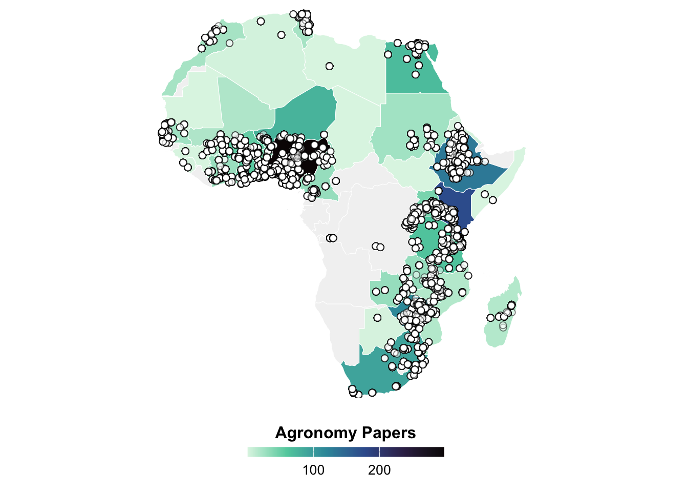
3.2 Exploring geographic locations of studies available

We collected country, site name paraphrased from study, and spatial coordinates when given. Location’s coordinates were verified in Google Maps, as they were often inaccurately reported. Enumerators also recorded a measure of spatial uncertainty. When authors reported decimal degrees and there was no correction required to the co-ordinates, then uncertainty was measured in terms of the value’s precision. When the location was estimated using Google Maps, the spatial uncertainty value was measured in terms of the precision of the site location description (e.g., a single farm or region) and the enumerator’s visual interpretation of land use at and near the coordinates. Observation’s geographic coordinates were collected to facilitate linking the data compiled in ERA to external databases, for example related to climatic and environmental factors not necessarily reported in the original study.

R code:

# Ensure coordinates are numeric
ERA.Compiled_ag <- ERA.Compiled_ag %>%
  mutate(
    Latitude = as.numeric(Latitude),
    Longitude = as.numeric(Longitude)
  ) %>%
  filter(!is.na(Latitude) & !is.na(Longitude))

# Count the number of papers per country
paper_counts <- ERA.Compiled_ag %>%
  group_by(Country) %>%
  summarise(N_Papers = n_distinct(Code), .groups = "drop")

# Load only African countries
world <- ne_countries(scale = "medium", continent = "Africa", returnclass = "sf")

# Fix Tanzania name if needed
world <- world %>%
  mutate(admin = if_else(admin == "United Republic of Tanzania", "Tanzania", admin))


# Ensure CRS is consistent
world <- st_transform(world, crs = 4326)

# Convert combined_sites to spatial data
sites_sf <- st_as_sf(ERA.Compiled_ag, coords = c("Longitude", "Latitude"), crs = 4326, remove = FALSE)

# Join paper counts to map
map_data <- world %>%
  dplyr::select(admin, geometry) %>%
  rename(Country = admin) %>%
  left_join(paper_counts, by = "Country")

# Plot the map
map<- ggplot() +
  geom_sf(data = map_data, aes(fill = N_Papers), color = "white") +
  geom_point(data = sites_sf, aes(x = Longitude, y = Latitude), 
             shape = 21, color = "black", fill = "white", size = 2, alpha = 0.5) +
  scale_fill_viridis_c(
    option = "mako",
    direction = -1,
    na.value = "gray95"
  ) +
  labs(fill = "Agronomy Papers") +
  theme_minimal() +
  theme(
    legend.position = "bottom",          # ⬅ Move to bottom
    legend.direction = "horizontal",     # ⬅ Make it horizontal
    legend.title = element_text(size = 12, face = "bold"),
    legend.text = element_text(size = 10),
    axis.text = element_blank(),
    axis.ticks = element_blank(),
    axis.title = element_blank(),
    panel.grid = element_blank()
  ) +
  guides(fill = guide_colorbar(
    barwidth = 10, barheight = 0.5, title.position = "top", title.hjust = 0.5
  )) +
  coord_sf(xlim = c(-20, 55), ylim = c(-35, 38), expand = FALSE)

# Display the map
map

python code:

# Python equivalent code:

import pandas as pd
import numpy as np
import geopandas as gpd
import matplotlib.pyplot as plt

# Ensure coordinates are numeric
ERA_Compiled_ag['Latitude'] = pd.to_numeric(ERA_Compiled_ag['Latitude'], errors='coerce')
ERA_Compiled_ag['Longitude'] = pd.to_numeric(ERA_Compiled_ag['Longitude'], errors='coerce')
ERA_Compiled_ag = ERA_Compiled_ag.dropna(subset=['Latitude', 'Longitude'])

# Count the number of papers per country
paper_counts = (
    ERA_Compiled_ag
    .groupby('Country')
    .agg(N_Papers=('Code', 'nunique'))
    .reset_index()
)

# Load only African countries using Natural Earth data
world = gpd.read_file(gpd.datasets.get_path('naturalearth_lowres'))
world = world[world['continent'] == 'Africa']

# Fix Tanzania name if needed
world['admin'] = world['admin'].replace("United Republic of Tanzania", "Tanzania")

# Ensure CRS is consistent
world = world.to_crs(epsg=4326)

# Convert ERA_Compiled_ag to spatial data
sites_sf = gpd.GeoDataFrame(
    ERA_Compiled_ag,
    geometry=gpd.points_from_xy(ERA_Compiled_ag['Longitude'], ERA_Compiled_ag['Latitude']),
    crs="EPSG:4326"
)

# Join paper counts to map: select only country names and geometry, rename and merge
map_data = world[['admin', 'geometry']].rename(columns={'admin': 'Country'})
map_data = map_data.merge(paper_counts, on='Country', how='left')

# Plot the map
fig, ax = plt.subplots(figsize=(10, 8))

# Plot African countries colored by N_Papers; missing values will appear in light gray
map_data.plot(
    column='N_Papers',
    ax=ax,
    edgecolor='white',
    cmap='viridis',
    missing_kwds={'color': 'gray95', 'edgecolor': 'white'}
)

# Plot site locations
sites_sf.plot(
    ax=ax,
    marker='o',
    color='white',
    edgecolor='black',
    markersize=50,
    alpha=0.5
)

# Set plot limits to match the original R code coordinates
ax.set_xlim(-20, 55)
ax.set_ylim(-35, 38)
ax.axis('off')

# Add legend (customization may be needed to mirror ggplot's style)
plt.legend(title='Agronomy Papers', loc='lower center', ncol=3)
plt.tight_layout()
plt.show()

3.3 Exploring the products of studies available

The Product.Subtype column in the ERA.Compiled_ag dataset contains the specific crop types examined in each study (e.g., "Maize", "Rice", "Wheat").

To accurately count how many unique studies (identified by Code) examined each crop, the following code processes and summarizes the data.

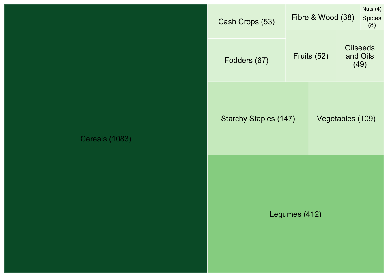
The figure below displays the distribution of crop categories in the dataset. It highlights the relative focus of studies across different crop types.

• The largest category by far is Cereals, indicating that most studies in ERA are focused on cereal crops such as maize, wheat, rice, and sorghum.

• This is followed by Legumes, Starchy Staples, and Vegetables, which also appear frequently in the dataset.

• Categories such as Fodders, Cash Crops, and Fruits are represented to a lesser extent.

Each tile represents a crop category, and its size reflects the number of unique studies (Code) that included at least one crop from that category. The number in parentheses shows the count of studies for that group.

R code:

prod_counts <- ERA.Compiled_ag %>%
  separate_rows(Product.Subtype, sep = "-") %>% 
  group_by(Product.Subtype) %>%
  summarise(Count = n_distinct(Code), .groups = "drop") %>%
  mutate(label = paste0(Product.Subtype, " (", Count, ")"))


tree_plot<- ggplot(prod_counts, aes(area = Count, fill = Count, label = label)) +
  geom_treemap(color = "white") +
  geom_treemap_text(
    colour = "black",
    place = "centre",
    grow = FALSE,       # Disable growing to avoid oversized text
    reflow = TRUE,
    size = 10            # Adjust this value to control the actual text size
  ) +
  scale_fill_distiller(palette = "Greens", direction = 1, guide = "none") +
  theme_minimal() +
  theme(
    plot.title = element_text(size = 14, face = "bold"),
    legend.position = "none"
  )
tree_plot

python code:

# Python equivalent code:
import pandas as pd
import squarify
import matplotlib.pyplot as plt

# Separate rows by "-" in the "Product.Subtype" column
prod_counts = (
    ERA_Compiled_ag
    .assign(Product_Subtype=ERA_Compiled_ag['Product.Subtype'].str.split('-'))
    .explode('Product_Subtype')
    .groupby('Product_Subtype')
    .agg(Count=('Code', 'nunique'))
    .reset_index()
)

# Create label as "Product.Subtype (Count)"
prod_counts['label'] = prod_counts['Product_Subtype'] + " (" + prod_counts['Count'].astype(str) + ")"

# Plot the treemap
plt.figure(figsize=(10, 8))
sizes = prod_counts['Count'].values
labels = prod_counts['label'].values

# Normalize sizes for colormap mapping
normed = sizes / sizes.max()
colors = plt.cm.Greens(normed)

squarify.plot(sizes=sizes, label=labels, color=colors, alpha=0.7)
plt.axis('off')
plt.title('Products Treemap', fontsize=14, fontweight='bold')

# Set white borders for each rectangle
for patch in plt.gca().patches:
    patch.set_linewidth(1)
    patch.set_edgecolor('white')

plt.show()

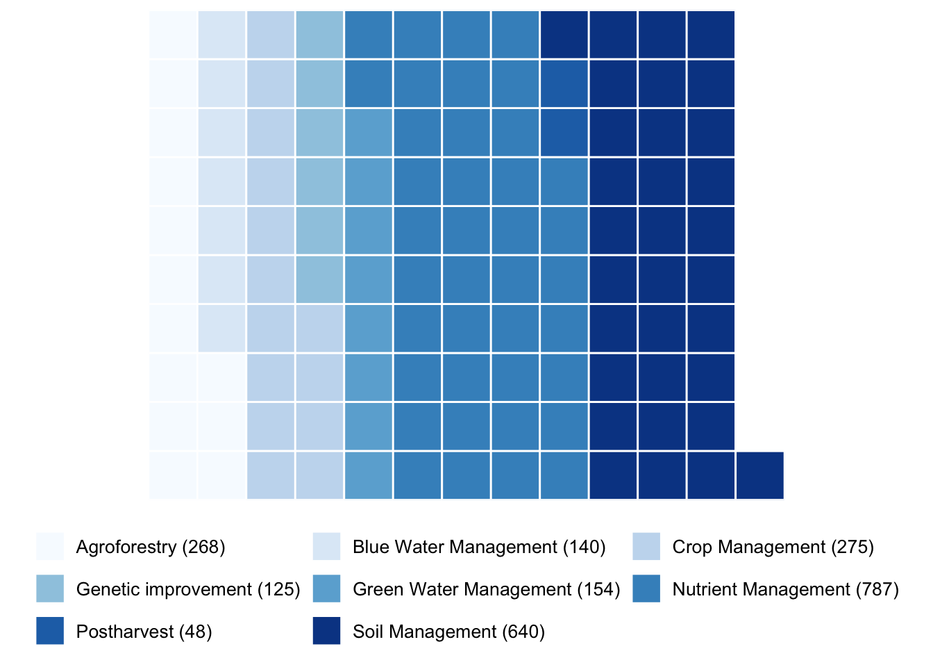
3.4 Exploring the agronomic practices within studies available

The following analysis explores the types of agronomic practices-referred to as “Themes” in the dataset.

Each study in ERA may be associated with multiple practices—for example, a study might examine both Soil Management and Nutrient Management.
For example, the theme ‘Soil Management’ include practices like green manure, crop residue, pH control, tillage, improved fallows. ‘Nutrient Management’ includes organic and inorganic fertilizer. This can be found in the practices within the mastercodes

R code:

ag_counts <- ERA.Compiled_ag %>%
  separate_rows(Theme, sep = "-") %>% 
  group_by(Theme) %>%
  summarise(Count = n_distinct(Code), .groups = "drop") %>%
  mutate(label = paste0(Theme, " (", Count, ")"))

# Define parts per square (e.g. 1 square = 10 studies)
parts_per_square <- 20

# Prepare waffle input
waffle_data <- ag_counts %>%
  mutate(
    squares = round(Count / parts_per_square)
  ) %>%
  filter(squares > 0)  # Drop any 0-square items

# Named vector for waffle
waffle_vec <- setNames(waffle_data$squares, waffle_data$label)

# Waffle plot
waffle_plot <- waffle::waffle(
  parts = waffle_vec,
  rows = 10,
  size = 0.5,
  colors = RColorBrewer::brewer.pal(n = nrow(waffle_data), name = "Blues"),
  legend_pos = "bottom"
) +
  theme(
    legend.position = "bottom",
    legend.text = element_text(size = 10),
    legend.title = element_blank()
  ) +
  guides(fill = guide_legend(nrow = 3, byrow = TRUE))

waffle_plot

python code:

# Python equivalent code:

import pandas as pd
import numpy as np
from pywaffle import Waffle
import matplotlib.pyplot as plt
import matplotlib as mpl

# Separate rows by "-" in the "Theme" column and count unique 'Code's
ag_counts = (
    ERA_Compiled_ag
    .assign(Theme=ERA_Compiled_ag['Theme'].str.split('-'))
    .explode('Theme')
    .groupby('Theme')
    .agg(Count=('Code', 'nunique'))
    .reset_index()
)
ag_counts['label'] = ag_counts['Theme'] + " (" + ag_counts['Count'].astype(str) + ")"

# Define parts per square (e.g. 1 square = 20 studies)
parts_per_square = 20

# Prepare waffle input: compute squares per theme
waffle_data = ag_counts.copy()
waffle_data['squares'] = (waffle_data['Count'] / parts_per_square).round().astype(int)
waffle_data = waffle_data[waffle_data['squares'] > 0]

# Create a dictionary for the waffle plot: keys are labels, values are squares
waffle_vec = dict(zip(waffle_data['label'], waffle_data['squares']))

# Generate a color palette similar to RColorBrewer "Blues"
n_categories = len(waffle_data)
colors = [mpl.cm.Blues(i) for i in np.linspace(0.3, 0.7, n_categories)]

# Plot the waffle chart
fig = plt.figure(
    FigureClass=Waffle,
    rows=10,
    values=waffle_vec,
    colors=colors,
    legend={
        'loc': 'lower center',
        'bbox_to_anchor': (0.5, -0.1),
        'ncol': 3,
        'fontsize': 10
    },
    title={'label': 'Practices Waffle Chart', 'loc': 'center'},
    figsize=(10, 8)
)

plt.show()

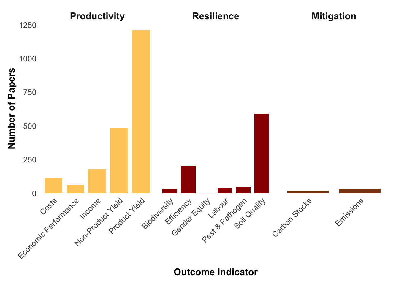
3.5 Exploring outcomes reported in the studies available

The ERA dataset tracks outcomes of agronomic interventions across several broad categories—called Pillars—such as productivity, environmental impact, and more. Each pillar includes more specific indicators like yield, GHG emissions, soil organic carbon, and others.

R code:

# Aggregate data by pillar and indicator
out_counts <- ERA.Compiled_ag %>%
  mutate(Out.Pillar = trimws(as.character(Out.Pillar))) %>%
  filter(Out.Pillar != "", !is.na(Out.Pillar), !is.na(Out.Ind)) %>%
  group_by(Out.Pillar, Out.Ind) %>%
  summarise(Num_Papers = n_distinct(Code), .groups = "drop") %>%
  rename(Pillar = Out.Pillar, Indicator = Out.Ind)


# Sort indicators within each pillar
out_counts <- out_counts %>%
  arrange(Pillar, Indicator) %>%
  mutate(
    Indicator = factor(Indicator, levels = unique(Indicator)),
    Pillar = factor(Pillar, levels = c("Productivity", "Resilience", "Mitigation"))
  )

# Optional: define pillar colors
pillar_colors <- c(
  "Productivity" = "#FFCC66",
  "Resilience" = "#990000",
  "Mitigation" = "#8B4513"
)

# Plot
bar_plot <- ggplot(out_counts, aes(
  x = Indicator, y = Num_Papers, fill = Pillar
)) +
  geom_col(width = 0.8) +
  labs(
    y = "Number of Papers",
    x = "Outcome Indicator"
  ) +
  scale_fill_manual(values = pillar_colors, na.value = "gray70") +
  scale_y_continuous(
    limits = c(0, max(out_counts$Num_Papers) + 50),
    expand = c(0, 0)
  ) +
  facet_wrap(~Pillar, scales = "free_x", nrow = 1) +
  theme_minimal() +
  theme(
    axis.text.x = element_text(size = 10, angle = 45, hjust = 1),
    axis.text.y = element_text(size = 10),
    axis.title.x = element_text(size = 12, face = "bold", margin = margin(t = 10)),
    axis.title.y = element_text(size = 12, face = "bold"),
    legend.position = "none",
    panel.grid.major = element_blank(),
    panel.grid.minor = element_blank(),
    strip.text = element_text(size = 12, face = "bold"),
    plot.margin = margin(10, 10, 10, 10)
  )

# Show plot
bar_plot

python code:

# Python equivalent code:

import pandas as pd
import numpy as np
import matplotlib.pyplot as plt
import seaborn as sns

# Aggregate data by pillar and indicator
# Trim whitespace from 'Out.Pillar' and filter out empty/missing values
out_counts = ERA_Compiled_ag.copy()
out_counts['Out.Pillar'] = out_counts['Out.Pillar'].astype(str).str.strip()
out_counts = out_counts[
    (out_counts['Out.Pillar'] != "") &
    (out_counts['Out.Pillar'].notna()) &
    (out_counts['Out.Ind'].notna())
]

# Group by Out.Pillar and Out.Ind, counting unique 'Code'
out_counts = (
    out_counts.groupby(['Out.Pillar', 'Out.Ind'], as_index=False)
    .agg(Num_Papers=('Code', 'nunique'))
)

# Rename columns: Pillar = Out.Pillar, Indicator = Out.Ind
out_counts = out_counts.rename(columns={'Out.Pillar': 'Pillar', 'Out.Ind': 'Indicator'})

# Sort indicators within each pillar
out_counts = out_counts.sort_values(by=['Pillar', 'Indicator'])

# Set categorical ordering:
# For Indicator, levels are based on order of appearance
indicator_levels = out_counts['Indicator'].unique().tolist()
out_counts['Indicator'] = pd.Categorical(out_counts['Indicator'], categories=indicator_levels, ordered=True)
# For Pillar, use a fixed order
pillar_order = ["Productivity", "Resilience", "Mitigation"]
out_counts['Pillar'] = pd.Categorical(out_counts['Pillar'], categories=pillar_order, ordered=True)

# Define pillar colors
pillar_colors = {
    "Productivity": "#FFCC66",
    "Resilience": "#990000",
    "Mitigation": "#8B4513"
}

# Create faceted bar plot: one subplot per Pillar
pillars = [p for p in pillar_order if p in out_counts['Pillar'].cat.categories]
num_pillars = len(pillars)
fig, axes = plt.subplots(1, num_pillars, figsize=(5 * num_pillars, 5), sharey=False)

# Ensure axes is iterable when only one subplot exists
if num_pillars == 1:
    axes = [axes]

for ax, pillar in zip(axes, pillars):
    subset = out_counts[out_counts['Pillar'] == pillar]
    ax.bar(subset['Indicator'], subset['Num_Papers'],
           color=pillar_colors.get(pillar, "gray70"), width=0.8)
    ax.set_xlabel("Outcome Indicator", fontsize=12, fontweight='bold', labelpad=10)
    ax.set_ylabel("Number of Papers", fontsize=12, fontweight='bold')
    ax.tick_params(axis='x', labelsize=10, rotation=45)
    ax.tick_params(axis='y', labelsize=10)
    ax.set_ylim(0, subset['Num_Papers'].max() + 50)
    ax.set_title(pillar, fontsize=12, fontweight='bold')
    # Remove grid and extra spines to mimic theme_minimal()
    ax.grid(False)
    ax.spines['top'].set_visible(False)
    ax.spines['right'].set_visible(False)

plt.tight_layout()
plt.show()

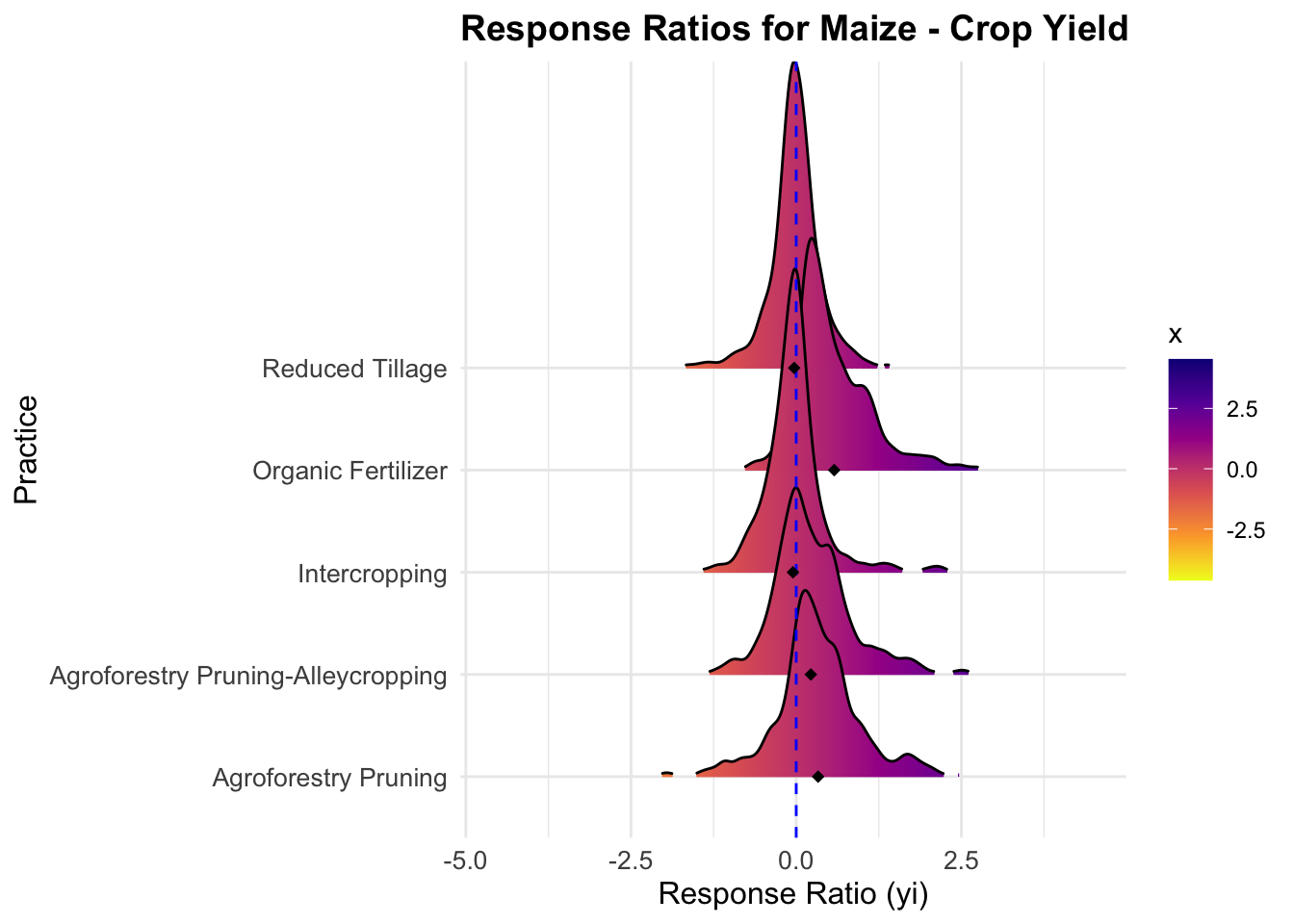
4 An example of an analysis you could do with ERA.Compiled

Lets assume you want to explore the impact of agriculture technologies on Maize yields. ERA only considers treatment comparisons. Each observation encodes a comparison between two treatments.

The following principles assisted in consistent comparisons of treatment outcomes across studies:

1. New versus common treatment. A new technology versus a control, which is typically farmers’ conventional technologies.

2. Additive complexity. An improved technology / set of technologies to a simpler option, e.g., agroforestry+fertilizer vs agroforestry alone.

3. Agriculture to agriculture. Agricultural systems are never compared to natural systems. For example, we can compare soil organic carbon in mulch versus no mulch systems, but not versus natural or semi-natural vegetation.

4. Same implementation levels. Comparisons were made within the same ‘level’ of implementation. For example, 40 kg N/ha was compared with other treatments using 40 kgN/ha but not 20 kgN/ha.

5. All treatment details. All major characteristics of the treatments were coded, including seed variety, tillage type, weed control, tree species, and chemical applications, among others, up to 13 labels per treatment.

6. In-year comparisons. Only comparisons of treatments and outcomes that occur in the same year or season were included. Residual effects, e.g., of phosphorus applied in year one with yield in year three, were not recorded.

7. Include all possible treatments. All treatments, and their component technologies, in a study were coded if they formed part of valid comparison.

Based this, a response ratio is calculated by MeanT/MeanC

R code:

filtered_data <- ERA.Compiled_ag %>%
  filter(Product == "Maize", Out.SubInd == "Crop Yield", !is.na(yi))

# Step 2: Keep only practices with at least 3 values and some variation
valid_practices <- filtered_data %>%
  group_by(PrName) %>%
  filter(n() >= 3, sd(yi, na.rm = TRUE) > 0) %>%
  ungroup()

# Step 3: Get top 5 PrName by number of rows
top_practices <- valid_practices %>%
  count(PrName, sort = TRUE) %>%
  slice_head(n = 5) %>%
  pull(PrName)

# Step 4: Final filtered data
ridge_data <- valid_practices %>%
  filter(PrName %in% top_practices)

# Step 5: Plot
ridge_plot <- ggplot(ridge_data, aes(x = yi, y = PrName, fill = ..x..)) +
  geom_density_ridges_gradient(scale = 3, rel_min_height = 0.01, color = "black") +
  geom_vline(xintercept = 0, linetype = "dashed", color = "blue") +
  stat_summary(
    aes(x = yi),
    fun = mean,
    geom = "point",
    color = "black",
    shape = 18,
    size = 2
  ) +
  scale_fill_viridis_c(option = "C", direction = -1) +
  labs(
    title = "Response Ratios for Maize - Crop Yield",
    x = "Response Ratio (yi)",
    y = "Practice"
  ) +
  theme_minimal() +
  theme(
    plot.title = element_text(face = "bold", size = 14),
    axis.text = element_text(size = 10),
    axis.title = element_text(size = 12)
  )


ridge_plot
#> Picking joint bandwidth of 0.0954

python code:

# Python equivalent code:

import pandas as pd
import numpy as np
import matplotlib.pyplot as plt
import joypy

# Step 1: Filter data for Product "Maize", Out.SubInd "Crop Yield", and non-missing yi
filtered_data = ERA_Compiled_ag[
    (ERA_Compiled_ag['Product'] == "Maize") &
    (ERA_Compiled_ag['Out.SubInd'] == "Crop Yield") &
    (ERA_Compiled_ag['yi'].notna())
].copy()

# Step 2: Keep only practices with at least 3 values and some variation in yi
def valid_group(df):
    return (len(df) >= 3) and (df['yi'].std(ddof=0) > 0)

valid_practices = filtered_data.groupby('PrName').filter(valid_group)

# Step 3: Get top 5 PrName by number of rows
top_practices = (valid_practices['PrName']
                 .value_counts()
                 .nlargest(5)
                 .index
                 .tolist())

# Step 4: Final filtered data
ridge_data = valid_practices[valid_practices['PrName'].isin(top_practices)].copy()

# Step 5: Plot ridgeline plot using joypy

# Compute the mean of yi for each practice for summary points
mean_values = ridge_data.groupby('PrName')['yi'].mean()

# Create the ridgeline plot
fig, axes = joypy.joyplot(
    ridge_data,
    by="PrName",
    column="yi",
    kind="kde",
    overlap=1,
    colormap=plt.cm.viridis,
    linewidth=1,
    linecolor="black",
    fade=True,
    figsize=(10, 6)
)

# Add a vertical dashed line at x = 0
plt.axvline(x=0, linestyle="dashed", color="blue")

# Add mean points for each practice
# Joypy orders groups alphabetically by default; get that order for accurate y positions
practices = sorted(ridge_data['PrName'].unique())
y_positions = {pr: i for i, pr in enumerate(practices)}
for pr, mean_val in mean_values.items():
    # The y position for each group corresponds to its index in the sorted list
    y = y_positions[pr]
    plt.plot(mean_val, y, marker="D", color="black", markersize=6)

plt.title("Response Ratios for Maize - Crop Yield", fontsize=14, fontweight="bold")
plt.xlabel("Response Ratio (yi)", fontsize=12, fontweight="bold")
plt.ylabel("Practice", fontsize=12, fontweight="bold")
plt.tight_layout()
plt.show()

5 The ERAg package

The ERAg R package was developed to support users working with an earlier version of the ERA.Compiled dataset (as of 2018). While the package has not been updated to reflect the latest additions to the dataset, it remains a useful resource for exploring functionality, accessing sample code, and understanding how to work with ERA’s comparisons table.

Although the comparison table included in the package is now out of date, many of the functions remain valid and may simplify analysis workflows using the more recent ERA.Compiled object loaded in this guide.

⚠️ Note: The package is written in R only. There is currently no Python version available.

We plan to update the ERAg package in the near future to reflect the latest data and metadata structures. Keep an eye on the GitHub repository for announcements.

5.1 ERAg vignettes

The ERAg R package provides a set of worked examples to help users explore, analyze, and better understand the ERA dataset. These vignettes illustrate key workflows and methods using the standardized ERA data model and should still be largely relevant to the more recent versions of ERA.Compiled stored on S3.

• ERA-Introduction
  Overview of the ERA dataset structure and access.
  This vignette introduces the main components of the ERAg package, such as the master sheet, comparisons table, and coded variables. It demonstrates how to load and inspect ERA data for meta-analysis.

• ERA-Explore-and-Analyze
  Basic workflows for summary statistics and visualization.
  Covers how to calculate treatment effects, filter observations by practice or outcome, and visualize impacts (e.g. on yield or soil organic carbon) using reproducible R code.

• ERA-Search-Protocol
  Systematic review methods and Boolean search strings.
  Details the structured search strategy used to compile the ERA dataset across Web of Science and Scopus (1970–2018), including practice and outcome keywords, inclusion criteria, and screening workflow.

• ERA-Yield-Stability
  Measuring long-term performance using stability metrics.
  Explains how to compute absolute and relative yield stability based on multi-year ERA data, inspired by methods from Knapp et al. (2018). Includes code for generating comparative stability plots.

6 Contact Us

Please visit our GitHub repository: https://github.com/ERAgriculture/ERA_Agronomy.git or our development GitHub: https://github.com/CIAT/ERA_dev

Or contact: Peter Steward (Scientist II): p.steward@cgiar.org
Namita Joshi (Senior Research Associate): n.joshi@cgiar.org
Todd Rosenstock (Principal Scientist): t.rosenstock@cgiar.org