Agroecological Agronomy Data in ERA (Maize, Bean & Coffee)

Author

Peter Steward & Namita Joshi (Alliance of Bioversity International & CIAT)

Published

June 16, 2025

1 Overview

This vignette introduces the agroecological agronomy dataset for the Agroecology in the Dry Corridor of Central America (ACDC) project, created using the Evidence for Resilient Agriculture (ERA) system.

The purpose of this document is to:

  • Provide open access to the ACDC dataset.
  • Facilitate exploration and use by researchers, analysts, and decision-makers.
  • Demonstrate current contents and structure.

For full background on ERA and its methods, see the ERA GitHub repository and the ERA User Guide.

For details on how climate and soils data are integrated into ERA, see the companion vignette: ERA Climate and Soils.

2 Set-up

2.1 Load Required Functions and Packages

2.2 Download ERA Data

# Set S3 path and initialize
s3 <- s3fs::S3FileSystem$new(anonymous = TRUE)

# This is the ERA s3 bucket
era_s3 <- "s3://digital-atlas/era"
# This is the S3 directory where era data archives can be found
(bundle_dir <- file.path(era_s3, "data", "packaged"))
[1] "s3://digital-atlas/era/data/packaged"
# This is the address of the most recent version of era agronomy
era_agronomy_s3<-"s3://digital-atlas/era/data/packaged/era_agronomy_bundle.tar.gz" 

# Create a folder to download the most recent version of era agronomy
dl_dir <- "downloaded_data"
dir.create(dl_dir, showWarnings = FALSE)

# Local file path of downloaded agronomy archive
(bundle_local <- file.path(dl_dir, basename(era_agronomy_s3)))
[1] "downloaded_data/era_agronomy_bundle.tar.gz"
# Name of folder to extract downloaded archive to
(extract_dir <- file.path(dl_dir, tools::file_path_sans_ext(tools::file_path_sans_ext(basename(era_agronomy_s3)))))
[1] "downloaded_data/era_agronomy_bundle"
if(update){
  # Download archive
  s3$file_download(era_agronomy_s3, bundle_local, overwrite = TRUE)
  
  # Extract archive
  dir.create(extract_dir)
  utils::untar(bundle_local, exdir = extract_dir)
  }

# Locate files
json_agronomic <- list.files(extract_dir, pattern = "^agronomic_.*\\.json$", full.names = TRUE)
json_master <- list.files(extract_dir, pattern = "^era_master_codes.*\\.json$", full.names = TRUE)
compiled_file <- list.files(extract_dir, pattern = "^era_compiled.*\\.parquet$", full.names = TRUE)

# Load the downloaded datasets
era_compiled <- arrow::read_parquet(compiled_file)
era_raw<- jsonlite::fromJSON(json_agronomic)
era_master_codes <- jsonlite::fromJSON(json_master)

3 Explore the Results

3.1 Treatment vs control comparisons

The downloaded era_compiled parquet table contains detailed information on control vs treatment comparisons. This is a large table with many fields.

dim(era_compiled)
[1] 197731    138

3.2 Field Names and Descriptions

How do we understand what these fields are? We can look at the era_master_codes to find the data catalog.

era_dat_fields <- era_master_codes$era_fields_v1 %>%
  select(Field, Display_Name, Field_Description)

era_dat_fields[1:5,]
          Field           Display_Name
1        B.Code   ERA Publication Code
2 B.Author.Last       Author Last Name
3        B.Date         Year Published
4     B.Journal                Journal
5         B.New New Journal Name Used?
                                            Field_Description
1 A unique publication code should be automatically assigned.
2                         Publication first author's surname.
3                                    The year of publication.
4              Name of journal this research is published in.
5                                                          NA

3.3 Subset to ACDC Region

The era compiled dataset contains information from multiple projects, so next we need to subset to the acdc project. We can do this by selecting data from central and south America.

lac_countries<-c("Ecuador","Brazil","Peru","Guatemala","Colombia","Venuezela","Costa Rica",
                 "Honduras","Nicaragua","Haiti","Mexico","El Salvador")
acdc_dat<-era_compiled[Country %in% lac_countries]

3.4 Summary Statistics

The subset data contains 16998 observations from 214 studies.

Lets explore what crops (Product.Simple), experimental management practices (PrName) and outcomes (Out.SubInd) we have in these data.

dat<-acdc_dat[,.(n_studies=length(unique(Code)),n_observations=.N),by=Product.Simple][order(n_studies,decreasing=T)]


kable(dat, format = "html", caption = "Studies and Observations by Crop") %>%
  kable_styling(full_width = FALSE) %>%
  scroll_box(width = "100%", height = "400px")
Studies and Observations by Crop
Product.Simple n_studies n_observations
Maize 111 3754
Wheat 29 4296
Soybean 23 2646
Common Bean 21 578
Coffee 16 287
Coffee-Natural Fallow 8 761
Arabica 6 195
Sorghum 5 238
Oats 5 208
Black oats 5 346
Durum Wheat 5 649
Common Bean-Maize 4 46
Black oats-Maize 4 27
Cowpea 4 67
Maize-Wheat 4 145
Maize-Natural Fallow 3 20
Macadamia 3 142
Arabica-Macadamia 3 614
Coffee-Macadamia 3 151
Barley 3 25
Natural Fallow 3 606
Cotton 2 37
Yacon 2 54
Palisade Grass 2 46
Hairy Vetch 2 8
Cowpea-Maize 2 25
Maize-Oats 2 102
Safflower 2 18
Capsicum 1 6
Groundnut-Maize 1 2
Coffee-Urochloa decumbens 1 6
Cabbage 1 3
Maize-Velvet Bean 1 2
Cabbage-Maize 1 4
Maize-Sunn Hemp 1 11
Guinea Grass 1 4
Sugar Cane 1 16
Sorghum-Soybean 1 66
Chamomile 1 34
Congo Grass-Cotton-Pearl Millet 1 180
Congo Grass 1 12
Guinea Grass-Soybean 1 1
Congo Grass-Soybean 1 1
Groundnut 1 24
Congo Grass-Maize-Soybean 1 18
Pearl Millet 1 4
Pigeon Pea 1 2
Maize-Pearl Millet-Pigeon Pea-Soybean 1 28
Black oats-Maize-Natural Fallow-Soybean-Wheat 1 1
Soybean-Wheat 1 1
Coffee-Rubber 1 8
Black oats-Guinea Grass-Maize-Soybean 1 54
Maize-Oats-Soybean-Wheat 1 36
Barley-Maize-Soybean-Wheat 1 6
Radish 1 6
Blue Lupin 1 6
Common Bean-Maize-Wheat 1 16
Hairy Vetch-Sorghum-Soybean-Wheat 1 2
Hairy Vetch-Maize-Soybean-Wheat 1 2
Black oats-Common Bean-Maize-Natural Fallow-Pearl Millet-Radish-Sunn Hemp 1 45
Black oats-Cowpea-Maize 1 12
Black oats-Maize-Oats-Soybean-Wheat 1 29
Melon 1 14
Grape 1 34
Napier Grass 1 15
Passionfruit 1 18
Sweet Potato 1 10
Sunflower 1 24
Opuntia stricta 1 15
Cassava 1 8
Horsegram-Maize 1 2
Hibiscus 1 48
Hibiscus-Maize 1 5
Common Bean-Hibiscus 1 5
Common Bean-Hibiscus-Maize 1 5
Maize-Pumpkin 1 2
Common Bean-Maize-Natural Fallow 1 4
Maize-Triticale 1 2
Fava Bean 1 5
Squash (C.Moschata) 1 5
Maize-Soybean 1 2
Maize-Peas 1 2
Common Bean-Wheat 1 8
Durum Wheat-Maize 1 26
# Note we will be exploring the impact of reducing or substituting inorganic fertilizers, so let's correct the practice name.
acdc_dat[,PrName:=gsub("Inorganic Fertilizer","Reduced Inorganic Fertilizer",PrName)]


dat<-acdc_dat[,.(n_studies=length(unique(Code)),n_observations=.N),by=.(PrName)][order(n_studies,decreasing=T)]

kable(dat, format = "html", caption = "Studies and Observations by Management Practice") %>%
  kable_styling(full_width = FALSE) %>%
  scroll_box(width = "100%", height = "400px")
Studies and Observations by Management Practice
PrName n_studies n_observations
Reduced Inorganic Fertilizer 82 2531
Reduced Tillage 32 5065
Intercropping 27 302
Organic Fertilizer 22 389
Crop Rotation 20 982
Mulch-Reduced Tillage 18 584
Mulch 18 968
pH Control 17 874
Multistrata Agroforestry 15 904
Crop Residue Incorporation 10 421
Reduced Inorganic Fertilizer-Organic Fertilizer 8 76
Crop Rotation-Reduced Tillage 7 51
Crop Rotation-Mulch-Reduced Tillage 6 74
Supplemental Irrigation 5 231
Reduced Inorganic Fertilizer-Intercropping 5 64
Crop Rotation-Mulch 5 54
Crop Rotation-Reduced Inorganic Fertilizer 4 16
Crop Residue Incorporation-Crop Rotation 4 38
Improved Fallow 3 182
Reduced Inorganic Fertilizer-pH Control 3 154
Other Agroforestry 3 64
Crop Residue Incorporation-Reduced Tillage 3 15
Improved Varieties 3 279
Reduced Inorganic Fertilizer-Mulch-Reduced Tillage 3 78
Reduced Inorganic Fertilizer-Mulch 3 111
Crop Residue 3 242
Crop Residue Incorporation-Mulch-Reduced Tillage 2 28
Improved Fallow-Intercropping 2 240
Double Cropping 2 17
Improved Varieties-Intercropping 2 10
Deficit Irrigation 2 178
Biochar 2 76
Alleycropping 2 396
Agroforestry Pruning 2 32
Biochar-Organic Fertilizer 2 31
Crop Residue-Reduced Tillage 2 42
Crop Residue-Intercropping-Reduced Tillage 2 8
Agroforestry Pruning-Multistrata Agroforestry 2 19
Green Manure 2 27
Harvest Method-Intercropping-Mulch 1 21
Crop Rotation-Intercropping-Reduced Tillage 1 1
Intercropping-Supplemental Irrigation 1 1
Improved Fallow-Reduced Inorganic Fertilizer 1 2
Improved Fallow-Reduced Inorganic Fertilizer-Intercropping 1 2
Agroforestry Pruning-Mulch 1 8
Agroforestry Pruning-Mulch-pH Control 1 4
Improved Varieties-pH Control 1 30
Improved Varieties-Reduced Inorganic Fertilizer-pH Control 1 120
Intercropping-Mulch 1 14
Multistrata Agroforestry-Supplemental Irrigation 1 26
Reduced Inorganic Fertilizer-Multistrata Agroforestry-pH Control 1 142
Reduced Inorganic Fertilizer-Multistrata Agroforestry 1 288
Biochar-Reduced Inorganic Fertilizer-Organic Fertilizer 1 10
Crop Rotation-Reduced Inorganic Fertilizer-Mulch 1 3
Crop Residue Incorporation-Crop Rotation-Mulch-Reduced Tillage 1 12
Organic Fertilizer-pH Control 1 16
Improved Varieties-Multistrata Agroforestry 1 8
Mulch-pH Control 1 3
Crop Rotation-pH Control 1 4
pH Control-Reduced Tillage 1 4
Alleycropping-Crop Rotation 1 4
Crop Rotation-Intercropping 1 8
Crop Rotation-Reduced Inorganic Fertilizer-Intercropping 1 4
Parklands 1 4
Mulch-Organic Fertilizer 1 2
Agroforestry Pruning-Alleycropping 1 48
Agroforestry Pruning-Alleycropping-Reduced Inorganic Fertilizer 1 24
Agroforestry Pruning-Organic Fertilizer 1 30
Crop Residue Incorporation-Mulch 1 26
Crop Residue-Intercropping 1 2
Other Agroforestry-Parklands 1 95
Intercropping-Reduced Tillage 1 4
Improved Varieties-Reduced Inorganic Fertilizer-Intercropping 1 6
Agroforestry Pruning-Reduced Inorganic Fertilizer 1 18
Crop Residue-Crop Rotation-Reduced Tillage 1 10
Biochar-Mulch-Organic Fertilizer 1 3
Biochar-Reduced Inorganic Fertilizer-Mulch-Organic Fertilizer 1 1
Crop Residue-Mulch 1 76
Crop Residue Incorporation-Reduced Inorganic Fertilizer 1 6
Reduced Inorganic Fertilizer-Reduced Tillage 1 4
Crop Residue-Mulch-Reduced Tillage 1 36
Agroforestry Pruning-Reduced Tillage 1 2
Green Manure-Reduced Inorganic Fertilizer 1 3
Green Manure-Organic Fertilizer 1 3
Green Manure-Reduced Inorganic Fertilizer-Organic Fertilizer 1 2
Crop Rotation-Organic Fertilizer 1 3
Crop Rotation-Reduced Inorganic Fertilizer-Organic Fertilizer 1 2
dat<-acdc_dat[,.(n_studies=length(unique(Code)),n_observations=.N),by=.(Out.SubInd)][order(n_studies,decreasing=T)]

kable(dat, format = "html", caption = "Studies and Observations by Outcome") %>%
  kable_styling(full_width = FALSE) %>%
  scroll_box(width = "100%", height = "400px")
Studies and Observations by Outcome
Out.SubInd n_studies n_observations
Crop Yield 170 5254
Biomass Yield 44 1046
Soil Organic Carbon 21 422
Gross Return 19 527
Soil Moisture 17 2749
Cation Exchange Capacity 13 199
Soil Total Nitrogen 11 242
Soil Organic Matter 10 138
Variable Cost 10 353
Total Cost 9 435
Crop Residue Yield 8 103
Biodiversity 8 974
Net Return 8 137
Water Use Efficiency 7 124
Nitrous Oxide Emissions 7 250
Soil Carbon Stocks 7 43
Gross Margin 6 140
Nitrogen Agronomic Efficiency 5 59
Erosion 3 22
Aboveground Carbon Biomass 3 26
Soil Nitrogen 2 58
Labour Person Hours 2 14
Soil NH4 2 117
Soil NO3 2 119
Fixed Cost 2 44
Belowground Carbon Biomass 2 2
Phosphorus Agronomic Efficiency 2 38
Carbon Dioxide Emissions 2 3076
Labour Cost 1 3
Effective Cation Exchange Capacity 1 30
Potassium Agronomic Efficiency 1 2
Nitrogen Agronomic Efficiency (AGB) 1 4
Nitrogen Use Efficiency (ARE AGB) 1 15
Phosphorus Use Efficiency (ARE AGB) 1 15
Potassium Use Efficiency (ARE AGB) 1 15
Benefit Cost Ratio (NRTC) 1 8
Total Cost (Unconfirmed) 1 13
Methane Emissions 1 100
Water Use 1 8
Runoff 1 18
Soil Organic Carbon (Change) 1 22
Infiltration Rate 1 8
Soil Available Nitrogen 1 16
Nitrogen Use Efficiency (Isotopic Product) 1 2
Nitrogen Use Efficiency (Isotopic AGB) 1 2
Benefit Cost Ratio (Unspecified) 1 6

3.5 Study Locations Map

# Ensure coordinates are numeric
acdc_dat <- acdc_dat %>%
  mutate(
    Latitude = as.numeric(Latitude),
    Longitude = as.numeric(Longitude)
  ) %>%
  filter(!is.na(Latitude) & !is.na(Longitude))

# Count and order papers by country (descending)
paper_counts <- acdc_dat %>%
  group_by(Country) %>%
  summarise(N_Papers = n_distinct(Code), .groups = "drop") %>%
  arrange(desc(N_Papers))  

# Load only Latin American countries and fix naming
world <- ne_countries(scale = "medium", continent = NULL, returnclass = "sf") %>%
  filter(continent %in% c("South America", "North America")) %>%
  # Fix country names to match your data if needed
  mutate(admin = case_when(
    admin == "United States of America" ~ "USA",
    admin == "Dominican Republic" ~ "Dominican Rep.",
    TRUE ~ admin
  ))

# Transform CRS
world <- st_transform(world, crs = 4326)

# Convert points to sf object
sites_sf <- st_as_sf(acdc_dat, coords = c("Longitude", "Latitude"), crs = 4326, remove = FALSE)

# Prepare map data
map_data <- world %>%
  dplyr::select(admin, geometry) %>%
  rename(Country = admin) %>%
  left_join(paper_counts, by = "Country")

# ---- Create map ----
map <- ggplot() +
  geom_sf(data = map_data, aes(fill = N_Papers), color = "white") +
  geom_point(data = sites_sf, aes(x = Longitude, y = Latitude), 
             shape = 21, color = "black", fill = "white", size = 2, alpha = 0.5) +
  scale_fill_viridis_c(
    option = "mako",
    direction = -1,
    na.value = "gray95"
  ) +
  labs(fill = "Number of experiments in ERA") +  # Changed legend title
  theme_minimal() +
  theme(
    legend.position = "bottom",
    legend.direction = "horizontal",
    legend.title = element_text(size = 12, face = "bold"),
    legend.text = element_text(size = 10),
    axis.text = element_blank(),
    axis.ticks = element_blank(),
    axis.title = element_blank(),
    panel.grid = element_blank()
  ) +
  guides(fill = guide_colorbar(
    barwidth = 10, barheight = 0.5, title.position = "top", title.hjust = 0.5
  )) +
  coord_sf(xlim = c(-120, -30), ylim = c(-60, 35), expand = FALSE)  # Zoom to Latin America

# ---- Create static table grob ----
table_grob <- tableGrob(head(paper_counts, 20))  


# ---- Plot map and table side by side ----
grid.arrange(map, table_grob, ncol = 2, widths = c(2, 1))

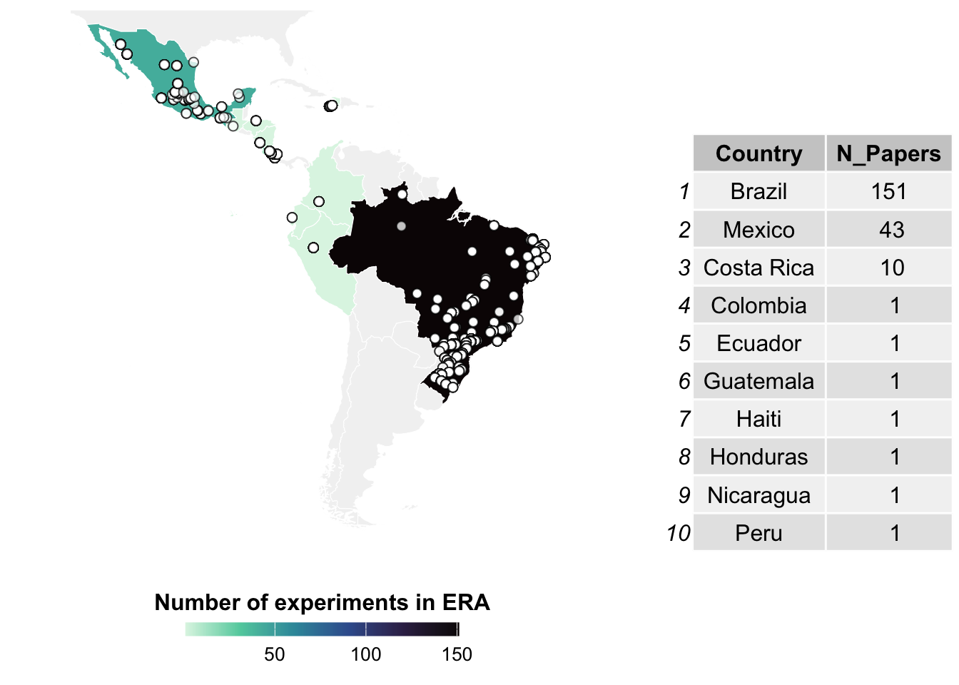
3.5.0.1 The total number of studies in countries within the Dry Corridor of Central America (Costa Rica, Guatemala, Honduras and Nicaragua) are a total of 13 papers.

3.6 Intersections of Factors

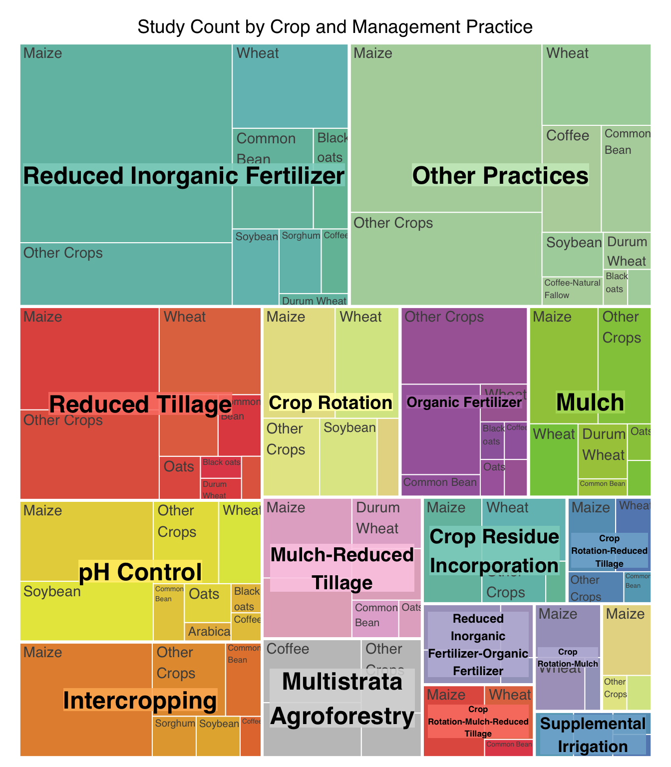
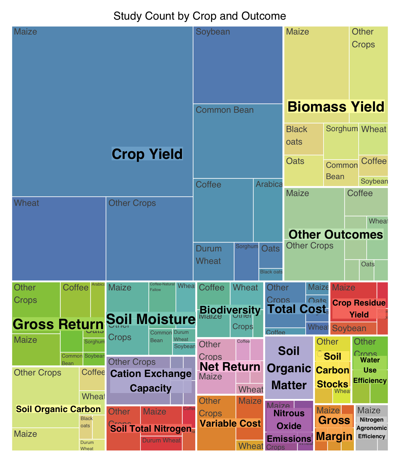
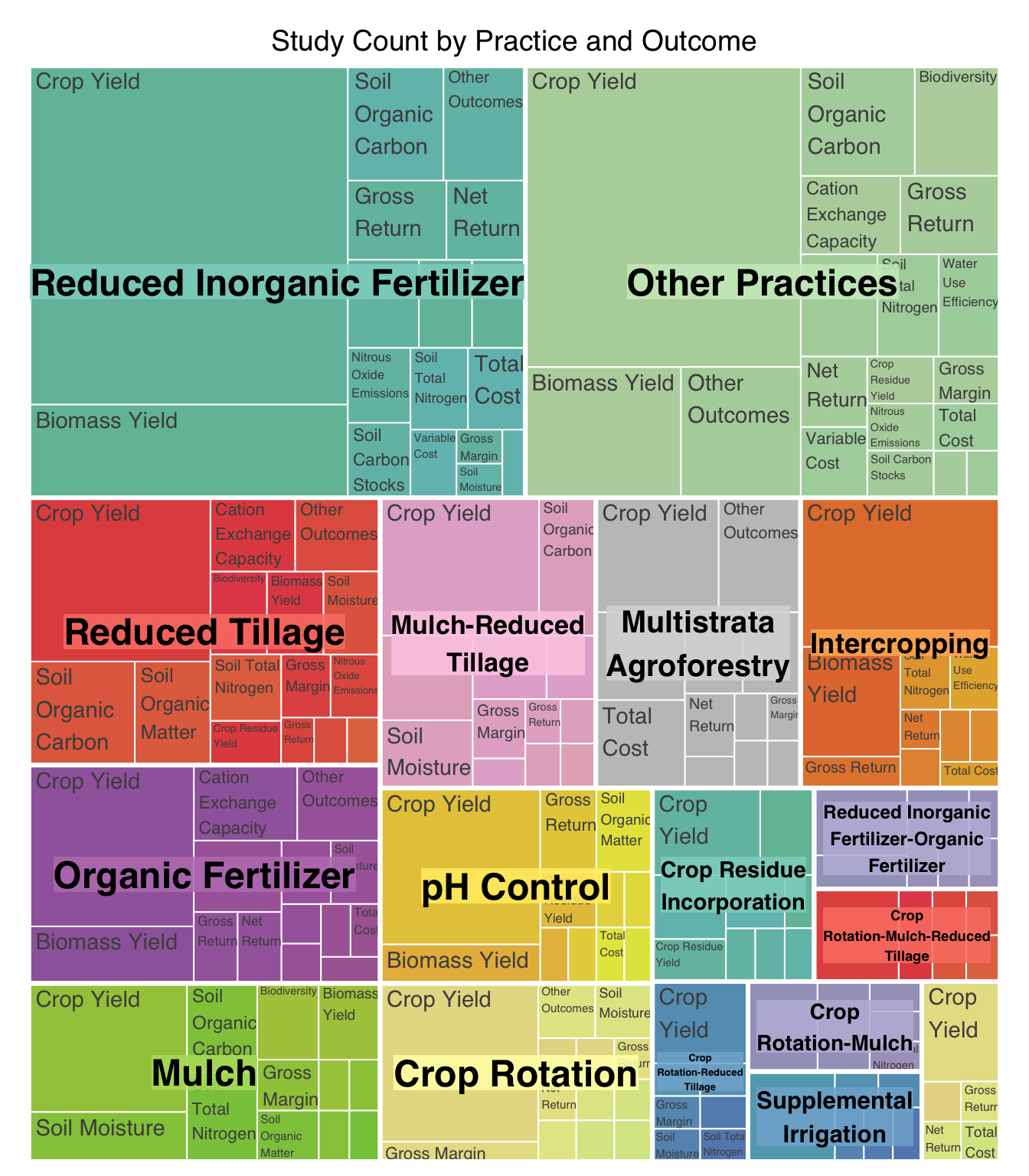
Lets look at the intersection of crops with practices, crops with outcomes, and outcomes with practices.

plot_dat<-copy(acdc_dat)[,Studies_crop:=length(unique(Code)),by=Product.Simple
                         ][,Studies_prac:=length(unique(Code)),by=PrName
                         ][Studies_crop<5,Product.Simple:="Other Crops"
                           ][Studies_prac<5,PrName:="Other Practices"
                           ][,.(Studies=length(unique(Code))),by=.(PrName,Product.Simple)]
library(treemap)

treemap(
  plot_dat,
  index = c("PrName","Product.Simple"),  # Crop first, then practice
  vSize = "Studies",
  title = "Study Count by Crop and Management Practice",
  palette = "Set3",
  border.col = "white",
  fontsize.labels = c(18, 11),      # Crop = bigger, practice = smaller
  fontcolor.labels = c("black", "grey30"),
  fontface.labels = c(2, 1),
  align.labels = list(c("center", "center"), c("left", "top")),
  drop.unused.levels = TRUE
)

plot_dat<-copy(acdc_dat)[,Studies_crop:=length(unique(Code)),by=Product.Simple
                         ][,Studies_out:=length(unique(Code)),by=Out.SubInd
                         ][Studies_crop<5,Product.Simple:="Other Crops"
                           ][Studies_out<5,Out.SubInd:="Other Outcomes"
                           ][,.(Studies=length(unique(Code))),by=.(Out.SubInd,Product.Simple)]

treemap(
  plot_dat,
  index = c("Out.SubInd","Product.Simple"),  # Crop first, then practice
  vSize = "Studies",
  title = "Study Count by Crop and Outcome",
  palette = "Set3",
  border.col = "white",
  fontsize.labels = c(18, 11),      # Crop = bigger, practice = smaller
  fontcolor.labels = c("black", "grey30"),
  fontface.labels = c(2, 1),
  align.labels = list(c("center", "center"), c("left", "top")),
  drop.unused.levels = TRUE
)

plot_dat<-copy(acdc_dat)[,Studies_prac:=length(unique(Code)),by=PrName
                         ][,Studies_out:=length(unique(Code)),by=Out.SubInd
                         ][Studies_prac<5,PrName:="Other Practices"
                           ][Studies_out<5,Out.SubInd:="Other Outcomes"
                           ][,.(Studies=length(unique(Code))),by=.(Out.SubInd,PrName)]

treemap(
  plot_dat,
  index = c("PrName","Out.SubInd"),  # Crop first, then practice
  vSize = "Studies",
  title = "Study Count by Practice and Outcome",
  palette = "Set3",
  border.col = "white",
  fontsize.labels = c(18, 11),      # Crop = bigger, practice = smaller
  fontcolor.labels = c("black", "grey30"),
  fontface.labels = c(2, 1),
  align.labels = list(c("center", "center"), c("left", "top")),
  drop.unused.levels = TRUE
)

4 Data Model

The extracted, harmonized data in the compiled dataset comes from a rich data model that contains much more information about management and context.

4.1 Understand Field Definitions

The data model (the era_raw object we created earlier) contains a number of interconnected tables.

names(era_raw)
 [1] "Pub.Out"      "Site.Out"     "Soil.Out"     "ExpD.Out"     "Times.Out"   
 [6] "Times.Clim"   "Prod.Out"     "Var.Out"      "Till.Out"     "Plant.Out"   
[11] "Plant.Method" "PD.Codes"     "PD.Out"       "Fert.Out"     "Fert.Method" 
[16] "Fert.Comp"    "Chems.Code"   "Chems.AI"     "Chems.Out"    "Weed.Out"    
[21] "Res.Out"      "Res.Method"   "Res.Comp"     "Har.Out"      "pH.Out"      
[26] "pH.Method"    "Irrig.Codes"  "Irrig.Method" "WH.Out"       "AF.Out"      
[31] "AF.Trees"     "Other.Out"    "Base.Out"     "MT.Out"       "Int.Out"     
[36] "Rot.Out"      "Rot.Seq"      "Rot.Seq.Summ" "Out.Out"      "Data.Out"    

To understand what each table contains look at the data catalog in era_master_codes.

era_raw_tabls <- era_master_codes$era_fields_v2 %>%
  select(Table, Table_Description) %>% unique


kable(era_raw_tabls, format = "html", caption = "Data Catalog - Table Descriptions") %>%
  kable_styling(full_width = FALSE) %>%
  scroll_box(width = "100%", height = "400px")
Data Catalog - Table Descriptions
Table Table_Description
1 Pub.Out This table captures bibliographic information. Each publication is assigned a unique code in the B.Code field that acts a key field in all other extraction template tables.
12 Site.Out Here we record the geographic co-ordinates of where an experiment has taken place and the uncertainty associated with this. You can record multiple locations. For each site you can also capture general biophysical information about the site and the starting conditions that describe the soils of the site.
40 Soil.Out This section is used to record detailed soil properties at the beginning of an experiment, including texture, pH, nutrient content, and other relevant information. You can add several lines to the table where soil properties are reported for multiple depths. Don't record soil properties measured after an experiment has begun here.
47 ExpD.Out Experimental design information, such as plot size, layout and notes on historical management.
48 ExpD.Out NA
52 Times.Out NA
57 Times.Clim NA
63 Var.Out NA
73 Till.Out Record details of tillage (or no tillage) here. If you have a base practice of conventional tillage you cannot have reduced or no-tillage as an experimental practices and vice-versa. Ridge & Furrow is "Conventional" if there is no comparison to pratice with more intensive tillage (e.g. mouldboard plough), if it is compared to a more intensive tillage practice then it is recorded "Reduced".
74 Till.Out NA
87 Plant.Out Describe the planting methods and arrangements used. The planting and arrangement of intercrops is recorded here (if different from an equivalent monocrop).
88 Plant.Out NA
94 Fert.Out NA
112 Fert.Method Each row of this table represents a fertilizer application https://agrovoc.fao.org/browse/agrovoc/en/page/c_10795
131 Fert.Method NA
135 Chems.Out NA
154 Weed.Out Weeding Practices. This section is for physical weeding practices only, herbicide applications should be noted under the chemicals tab.
155 Weed.Out NA
161 Res.Out This tab is primarily for the addition of non-composted organic materials that DO NOT come from experimental crops, use the crop residue column in the Make.Trt, Intercrop or Rotation tabs to record residues from a preceeding season. Record mulching of compost or manure in the Nutrients practice tab.
162 Res.Out NA
173 Res.Method This table records details of exactly what organic residue is added, where it is from, how much is added, what happens to it and when it is added.
174 Res.Method NA
193 Res.Composition This table records the compostion of the residue materials.
194 Res.Composition NA
218 Har.Out Harvest practices
219 Har.Out NA
223 pH.Out pH amendments
224 pH.Out NA
225 pH.Out pH.Codes
228 pH.Method NA
237 WH.Out NA
245 Base.Out NA
247 MT.Out2;MT.Out NA
267 Int.Out NA
270 Rot.Seq NA
284 Rot.Levels NA
288 Out.Out NA
298 Out.Econ NA
307 AF.Out NA
315 AF.Trees NA
320 Other.Out NA
323 Data.Out NA
343 PD.Out NA

To find explanations of the fields in each table also use the data catalog.

era_raw_fields<- era_master_codes$era_fields_v2 %>%
  filter(Table=="Fert.Out") %>%
  select(Field, Display_Name, Field_Description)


kable(era_raw_fields, format = "html", caption = "Data Catalog - Field Descriptions (Fert.Out)") %>%
  kable_styling(full_width = FALSE) %>%
  scroll_box(width = "100%", height = "400px")
Data Catalog - Field Descriptions (Fert.Out)
Field Display_Name Field_Description
F.Level.Name Fertilizer Practice Name Choose a easy to recognize name for the fertilizer practice, you will use this name to reference it when building treatments later in the extraction process. Avoid using special characters.
F.Rate.Pracs Fertilizer Rate Practice rate or dosage of fertilizer application used in the study
F.Timing.Pracs Fertilizer Timing Practice timing of fertilizer application
F.Info.Pracs Fertilizer Precision Practice details about the precision of fertilizer application
F.Precision.Pracs Fertilizer Information Practice NA
F.Int Intercropping Only : Applied to specific crop or whole plot ? NA
F.NO Total Organic Elemental N Total elemental nitrogen applied from organic sources (e.g., compost, manure, biosolid).
F.PO Total Organic Elemental P Total elemental phosphorus applied from organic sources (e.g., compost, manure, biosolid).
F.KO Total Organic Elemental K Total elemental potassium applied from organic sources (e.g., compost, manure, biosolid).
F.NI Total Inorganic Elemental N Total elemental nitrogen applied from inorganic sources (e.g., urea or DAP).
F.PI Total Inorganic Elemental P Total elemental phosphorus applied from inorganic sources (e.g., rock phosphate or DAP).
F.P2O5 Total Organic Elemental P2O5 Total phosphorus applied from inorganic sources presented as phosphorus pentoxide (P2O5) .
F.KI Total Organic Elemental K Total elemental potassium applied from inorganic sources (e.g., potassium chloride or monopotassium phosphate).
F.K2O Total Organic Elemental K Total potassium applied from inorganic sources presented as potassium oxide (K2O).
F.O.Unit Organic NPK Unit of Measurement The unit of measurement for total organic NPK numbers.
F.I.Unit Inorganic NPK Unit of Measurement The unit of measurement for total organic NPK numbers.
F.Notes Notes NA
B.Code NA A unique code that identifies an extracted publication in the ERA dataset. This code is present in all the tables of era extraction data models.

For more information on the ERA agronomy data model including table linkages and relational structure see.

4.2 Subset Raw Data for ACDC

acdc_raw_dat<-era_raw$Data.Out %>% filter(Country %in% lac_countries) %>% data.table

This gives us 11495 observations from 236.

This raw data is passed through complex comparison logic to select valid control vs experimental treatment comparisons. The R-code for the comparisons can be found here.

The number of extracted papers is less than the comparisons table as some extractions did not contain valid comparisons or have an extremely complicate structure beyond the capcacity of the comparison logic.

5 Literature Search and Screening

For transparency, search and screening documentation includes:

  1. Search terms

  2. Search results

  3. Screening results

screening<-fread("https://raw.githubusercontent.com/CIAT/ERA_dev/refs/heads/main/search_history/era-search-history.csv")

ta_pass<-screening$`title-abstract_pass`

We screened 7615 references, 2600 references passed title and abstract screening, 628 passed fulltext screening, and 211 papers were suitable for extraction into the final dataset.

We did not have access to 32 publications.

6 Next steps

  1. Climate Data Integration:
    • Merge ERA agronomic data with seasonal climate statistics.
    • For annual crops (maize, bean), experienced climate is calculated using planting date estimates.
    • For perennials (coffee), we are developing a new method to define yield-relevant climate exposure.
  2. Hazard–Management Intersection:
    • Once climate data is merged, we will explore if management practices influence outcomes under climate stress (e.g., drought, heat).
  3. Fertilizer Comparison Logic:
    • Identify experiments with multiple fertilizer levels.
    • Define comparisons for low vs moderate, moderate vs high, and low vs high fertilizer use.
    • Integrate these comparisons into ERA’s analysis logic.
  4. Meta-analysis of Practices:
    • Run meta-analysis on selected practices to assess their productivity and resilience benefits.
    • Focus on agroecological interventions in maize, bean, and coffee systems.